The format of data marker in a line, scatter and radar chart can be changed and customized, which makes it more attractive and distinguishable. We could set markers' built-in type, size, background color, foreground color and transparency in Excel. This article is going to introduce how to achieve those features in C# using Spire.XLS.
Note: before start, please download the latest version of Spire.XLS and add the .dll in the bin folder as the reference of Visual Studio.
Step 1: Create a workbook with sheet and add some sample data.
            Workbook workbook = new Workbook();
            workbook.CreateEmptySheets(1);
            Worksheet sheet = workbook.Worksheets[0];
            sheet.Name = "Demo";
            sheet.Range["A1"].Value = "Tom";
            sheet.Range["A2"].NumberValue = 1.5;
            sheet.Range["A3"].NumberValue = 2.1;
            sheet.Range["A4"].NumberValue = 3.6;
            sheet.Range["A5"].NumberValue = 5.2;
            sheet.Range["A6"].NumberValue = 7.3;
            sheet.Range["A7"].NumberValue = 3.1;
            sheet.Range["B1"].Value = "Kitty";
            sheet.Range["B2"].NumberValue = 2.5;
            sheet.Range["B3"].NumberValue = 4.2;
            sheet.Range["B4"].NumberValue = 1.3;
            sheet.Range["B5"].NumberValue = 3.2;
            sheet.Range["B6"].NumberValue = 6.2;
            sheet.Range["B7"].NumberValue = 4.7;
Step 2: Create a Scatter-Markers chart based on the sample data.
Chart chart = sheet.Charts.Add(ExcelChartType.ScatterMarkers);
chart.DataRange = sheet.Range["A1:B7"];
chart.PlotArea.Visible=false;
chart.SeriesDataFromRange = false;
chart.TopRow = 5;
chart.BottomRow = 22;
chart.LeftColumn = 4;
chart.RightColumn = 11;
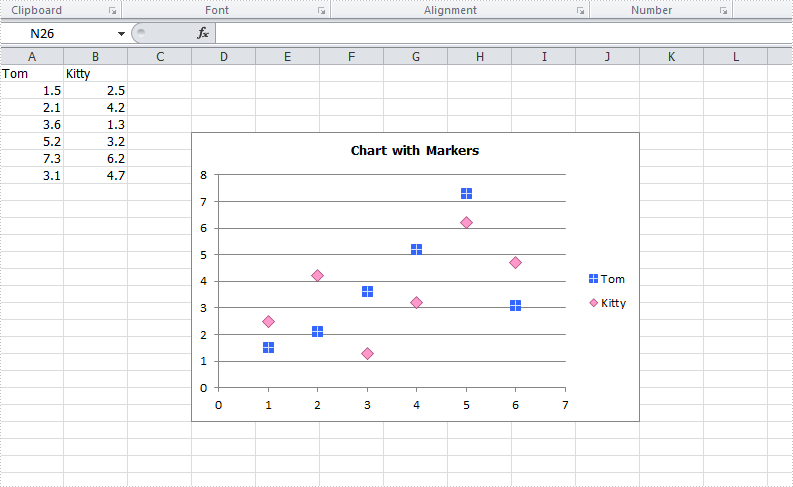
chart.ChartTitle = "Chart with Markers";
chart.ChartTitleArea.IsBold = true;
chart.ChartTitleArea.Size = 10;
Step 3: Format the markers in the chart by setting the background color, foreground color, type, size and transparency.
            Spire.Xls.Charts.ChartSerie cs1 = chart.Series[0];
            cs1.DataFormat.MarkerBackgroundColor = Color.RoyalBlue;
            cs1.DataFormat.MarkerForegroundColor = Color.WhiteSmoke;
            cs1.DataFormat.MarkerSize = 7;
            cs1.DataFormat.MarkerStyle = ChartMarkerType.PlusSign;
            cs1.DataFormat.MarkerTransparencyValue = 0.8;

            Spire.Xls.Charts.ChartSerie cs2 = chart.Series[1];
            cs2.DataFormat.MarkerBackgroundColor = Color.Pink;
            cs2.DataFormat.MarkerSize = 9;
            cs2.DataFormat.MarkerStyle = ChartMarkerType.Diamond;
            cs2.DataFormat.MarkerTransparencyValue = 0.9;
Step 4: Save the document and launch to see effects.
            workbook.SaveToFile("S3.xlsx", ExcelVersion.Version2010);
            System.Diagnostics.Process.Start("S3.xlsx");
Effects:
Full Codes:
using System;
using System.Collections.Generic;
using System.Linq;
using System.Text;
using Spire.Xls;
using System.Drawing;

namespace ConsoleApplication2
{
    class Program
    {
        static void Main(string[] args)
        {

            Workbook workbook = new Workbook();
            workbook.CreateEmptySheets(1);
            Worksheet sheet = workbook.Worksheets[0];

            sheet.Name = "Demo";
            sheet.Range["A1"].Value = "Tom";
            sheet.Range["A2"].NumberValue = 1.5;
            sheet.Range["A3"].NumberValue = 2.1;
            sheet.Range["A4"].NumberValue = 3.6;
            sheet.Range["A5"].NumberValue = 5.2;
            sheet.Range["A6"].NumberValue = 7.3;
            sheet.Range["A7"].NumberValue = 3.1;
            sheet.Range["B1"].Value = "Kitty";
            sheet.Range["B2"].NumberValue = 2.5;
            sheet.Range["B3"].NumberValue = 4.2;
            sheet.Range["B4"].NumberValue = 1.3;
            sheet.Range["B5"].NumberValue = 3.2;
            sheet.Range["B6"].NumberValue = 6.2;
            sheet.Range["B7"].NumberValue = 4.7;

            Chart chart = sheet.Charts.Add(ExcelChartType.ScatterMarkers);
            chart.DataRange = sheet.Range["A1:B7"];
            chart.PlotArea.Visible=false;
            chart.SeriesDataFromRange = false;
            chart.TopRow = 5;
            chart.BottomRow = 22;
            chart.LeftColumn = 4;
            chart.RightColumn = 11;
            chart.ChartTitle = "Chart with Markers";
            chart.ChartTitleArea.IsBold = true;
            chart.ChartTitleArea.Size = 10;

            Spire.Xls.Charts.ChartSerie cs1 = chart.Series[0];
            cs1.DataFormat.MarkerBackgroundColor = Color.RoyalBlue;
            cs1.DataFormat.MarkerForegroundColor = Color.WhiteSmoke;
            cs1.DataFormat.MarkerSize = 7;
            cs1.DataFormat.MarkerStyle = ChartMarkerType.PlusSign;
            cs1.DataFormat.MarkerTransparencyValue = 0.8;

            Spire.Xls.Charts.ChartSerie cs2 = chart.Series[1];
            cs2.DataFormat.MarkerBackgroundColor = Color.Pink;
            cs2.DataFormat.MarkerSize = 9;
            cs2.DataFormat.MarkerStyle = ChartMarkerType.Diamond;
            cs2.DataFormat.MarkerTransparencyValue = 0.9;

            workbook.SaveToFile("S3.xlsx", ExcelVersion.Version2010);
            System.Diagnostics.Process.Start("S3.xlsx");
        }
    }
}
