Как скопировать форматирование ячейки в Excel
Содержание
- Быстрое сравнение: выберите подходящий метод
- Копирование форматирования ячеек с помощью Формата по образцу
- Копирование форматирования ячеек с помощью специальной вставки
- Копирование форматирования ячеек с помощью маркера заполнения
- Повторное использование форматирования ячеек с помощью стилей ячеек
- Копирование правил условного форматирования в Excel
- Автоматическое копирование форматирования ячеек в Excel с помощью C#
- Устранение распространённых проблем с форматированием
- См. также
Когда новый раздел листа Excel должен соответствовать существующим ячейкам, копирование форматирования быстрее, чем повторное создание вручную. Можно повторно использовать шрифты, границы, цвет заливки, выравнивание и числовые форматы, не создавая каждый стиль заново.
Excel предлагает несколько способов копирования форматирования ячеек, включая Формат по образцу, Специальную вставку и маркер заполнения. Вы также можете использовать стили ячеек для поддержания единообразного форматирования во всей книге, копировать или расширять правила условного форматирования либо автоматизировать повторяющиеся задачи форматирования с помощью C#.
Быстрое сравнение: выберите подходящий метод
Используйте таблицу сравнения ниже, чтобы выбрать лучший метод для вашего рабочего процесса:
| Метод | Лучше всего подходит для | Ключевое преимущество |
|---|---|---|
| Формат по образцу | Быстрое копирование форматирования в несколько ячеек или несмежные диапазоны. | Наглядное форматирование всего за несколько щелчков. |
| Специальная вставка (Форматы) | Обновление больших диапазонов, уже содержащих данные или формулы. | Применяет форматирование, не перезаписывая существующее содержимое ячеек. |
| Маркер заполнения (Заполнить только форматы) | Расширение форматирования вниз по столбцу или по строке. | Быстрое форматирование перетаскиванием, с ярлыком двойного щелчка для заполнения вниз. |
| Стили ячеек | Поддержание единообразного форматирования во всей книге. | Централизованное управление; обновление стиля обновляет ячейки, использующие этот стиль. |
| Формат по образцу или Управление правилами | Копирование правил условного форматирования или их расширение на новые диапазоны данных. | Повторно использует существующие правила без их воссоздания. |
| Автоматизация на C# | Автоматизация крупномасштабных или повторяющихся задач форматирования. | Копирует форматирование программно, без ручного редактирования каждой книги. |
Копирование форматирования ячеек с помощью Формата по образцу
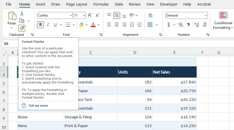
Формат по образцу копирует форматирование — например, шрифты, цвета заливки, границы, выравнивание и числовые форматы — не изменяя содержимое целевой ячейки. Этот инструмент хорошо подходит для быстрого применения существующего стиля к нескольким ячейкам или диапазонам.
Пошаговые инструкции
- Выберите ячейку или диапазон с форматированием, которое нужно скопировать.
- Перейдите на вкладку Главная > Формат по образцу в группе Буфер обмена.
- Щёлкните целевую ячейку или протяните по диапазону, который нужно отформатировать.
Полезные советы:
- Применение к нескольким областям: Дважды щёлкните Формат по образцу, чтобы оставить его активным. Это позволяет форматировать несколько несмежных ячеек или диапазонов. По завершении нажмите Esc, чтобы отключить его.
- Форматирование между книгами: Можно использовать Формат по образцу на разных листах или в разных книгах. Открыв обе книги в Excel, активируйте инструмент, переключитесь на целевой лист или книгу и выберите целевые ячейки.
Дополнительные сведения см. в руководстве Microsoft по копированию форматирования ячеек.
Копирование форматирования ячеек с помощью специальной вставки
Специальная вставка (Форматы) также позволяет копировать шрифты, цвета заливки, границы, выравнивание и числовые форматы из одной ячейки или диапазона в другой, не изменяя значения или формулы целевых ячеек.
Этот метод особенно полезен при применении форматирования к большим диапазонам или ячейкам, которые уже содержат данные.
Пошаговые инструкции
Выберите форматированные исходные ячейки и нажмите Ctrl + C (Windows) или Cmd + C (Mac).
Выберите верхнюю левую ячейку целевого диапазона. Если копируете форматирование одной ячейки в несколько ячеек, выберите весь целевой диапазон.
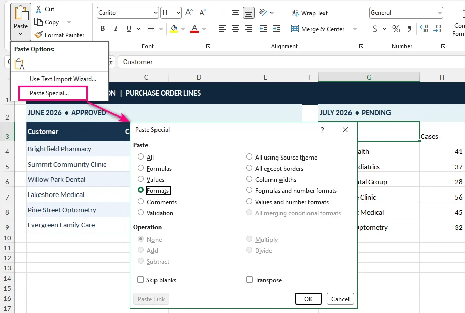
Перейдите на вкладку Главная, щёлкните стрелку под кнопкой Вставить и выберите Специальная вставка.
Выберите Форматы, затем нажмите ОК.
Полезные советы:
- Сочетания клавиш:
- Windows: Нажмите Ctrl + C, выберите целевой диапазон, затем нажмите Ctrl + Alt + V, T и Enter.
- Mac: Нажмите Cmd + C, выберите целевой диапазон, затем нажмите Ctrl + Cmd + V, чтобы открыть Специальную вставку. Выберите Форматы и подтвердите.
- Использование между книгами: Те же шаги работают на разных листах и в разных книгах. Держите оба файла Excel открытыми, скопируйте исходные ячейки, переключитесь на целевую книгу и примените Специальную вставку.
Важные моменты:
- Числовые форматы могут измениться: При этом числовые форматы копируются вместе с другими свойствами форматирования. Например, применение общего числового формата к ячейке с датой может привести к тому, что дата отобразится как её внутренний порядковый номер. При необходимости проверьте или повторно примените подходящий числовой формат после этого.
- Темы книг: При копировании между разными книгами окончательный вид шрифтов и цветов может измениться, если целевая книга использует другую тему Office.
Если вы хотите убедиться, что формулы в целевом диапазоне сохранились, см. раздел как просмотреть формулы в Excel.
Копирование форматирования ячеек с помощью маркера заполнения
При расширении таблицы в Excel можно использовать маркер заполнения, чтобы быстро скопировать форматирование существующей ячейки в соседние строки или столбцы без ручного воссоздания стилей.
Пошаговые инструкции
Выберите исходную ячейку, содержащую форматирование, которое нужно скопировать (например, D2).
Наведите курсор на маленький квадрат в правом нижнем углу ячейки, пока он не изменится на чёрный крестик (+).
Перетащите маркер заполнения вниз или в сторону до целевого диапазона (например, D3:D20).
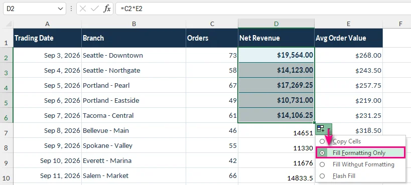
Нажмите кнопку Параметры автозаполнения, которая появится после отпускания мыши.
Выберите Заполнить только форматы.
Советы и рекомендации:
- Быстрое заполнение больших непрерывных диапазонов: Если соседний столбец содержит непрерывные данные, дважды щёлкните маркер заполнения, чтобы автоматически заполнить вниз вместо перетаскивания. Затем выберите Заполнить только форматы в меню Параметры автозаполнения.
- Используйте специальную вставку для существующих данных: Если целевые ячейки уже содержат важные формулы или данные, Специальная вставка (Форматы) безопаснее, поскольку применяет форматирование без копирования значений или формул.
Важное примечание:
- Маркер заполнения может изначально изменить содержимое ячеек: Перетаскивание маркера заполнения может заполнить значения или формулы вместе с форматированием, потенциально заменяя существующее содержимое ячеек. Если нужно скопировать только форматирование, выберите Заполнить только форматы сразу после заполнения.
Повторное использование форматирования ячеек с помощью стилей ячеек
Если вы часто применяете одно и то же форматирование к заголовкам отчётов, названиям разделов или промежуточным итогам, копирование форматирования из отдельных ячеек может стать утомительным. Функция стилей ячеек Excel позволяет создавать многоразовые наборы свойств форматирования для поддержания единообразия во всей книге.
Как создать и использовать настраиваемый стиль ячейки
Перейдите в Главная > Стили ячеек > Создать стиль ячейки.
Введите описательное имя стиля, например Заголовок отчёта или Финансовый итог.
Нажмите Формат и настройте шрифт, цвет заливки, границы, выравнивание и другие свойства форматирования.
В разделе Включаемые элементы стиля выберите атрибуты форматирования, которыми должен управлять стиль.
Нажмите ОК, чтобы сохранить новый стиль.
Выберите целевые ячейки и примените настраиваемый стиль из Главная > Стили ячеек.
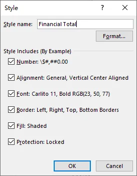
Советы:
- Обновление нескольких ячеек одновременно: При изменении существующего стиля ячейки изменения автоматически применяются ко всем ячейкам, использующим этот стиль, во всей книге.
- Сохранение числовых форматов: Если целевые ячейки содержат разные типы данных (например, даты, проценты или денежные значения), снимите флажок Число в разделе Включаемые элементы стиля на шаге 4. Это не позволит стилю изменять отображение этих значений.
- Повторное использование стилей в разных книгах: Вы можете перенести настраиваемые стили в другую книгу с помощью Главная > Стили ячеек > Объединить стили. Если обе книги содержат стили с одинаковым именем, Excel может спросить, заменять ли существующие стили в целевом файле.
Копирование правил условного форматирования в Excel
Условное форматирование изменяет внешний вид ячеек в зависимости от их значений или формул. Например, финансовый отчёт может отображать отрицательную прибыль красным цветом или выделять показатели продаж, превышающие целевое значение.
Вы можете копировать существующие правила условного форматирования с помощью Формата по образцу или расширить диапазон, охватываемый существующим правилом, с помощью Управления правилами.
Копирование условного форматирования с помощью Формата по образцу
Чтобы применить существующие правила условного форматирования к другой ячейке или диапазону:
- Выберите ячейку, содержащую условное форматирование, которое нужно скопировать.
- Перейдите в Главная > Формат по образцу.
- Выберите целевую ячейку или диапазон.
Скопированные правила оцениваются на основе используемых ими значений и ссылок на ячейки.
Примечание: Формат по образцу копирует обычное форматирование ячеек вместе с правилами условного форматирования. Если вы хотите только расширить существующее правило, не изменяя другие свойства форматирования, используйте следующий метод.
Расширение существующего правила условного форматирования с помощью Управления правилами
Предположим, правило условного форматирования выделяет отрицательную прибыль в D2:D10, и вы добавили новые строки, которые должны подчиняться тому же правилу.
Вместо многократного копирования правила можно расширить диапазон его применения.
Перейдите в Главная > Условное форматирование > Управление правилами.
Выберите правило, которое нужно изменить. При необходимости установите для параметра Показать правила форматирования для значение Этот лист.
В поле Применяется к измените диапазон с
=$D$2:$D$10на=$D$2:$D$20.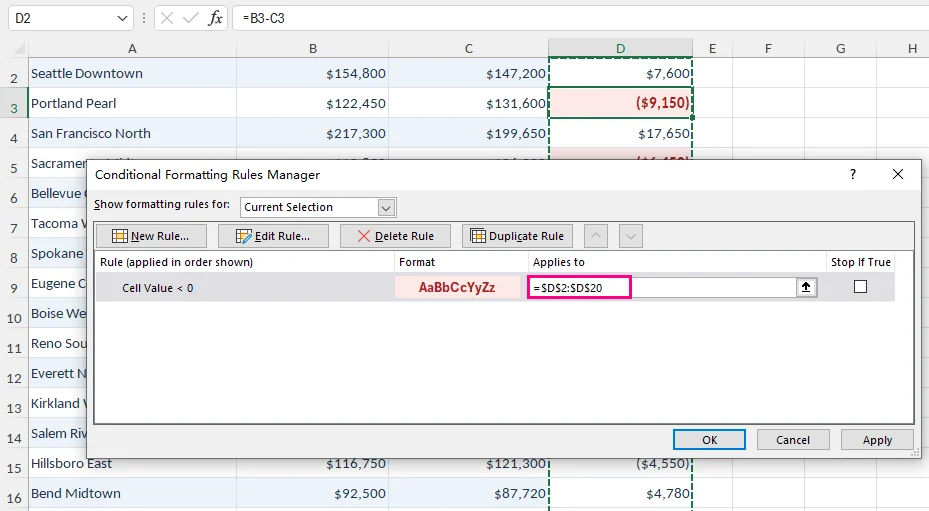
Нажмите Применить, затем ОК.
Теперь существующее правило охватывает дополнительные ячейки.
Совет: Если правило условного форматирования использует формулу, проверьте относительные и абсолютные ссылки на ячейки при копировании или расширении правила. Неправильные ссылки могут привести к тому, что форматирование будет вести себя иначе в новом диапазоне.
Вы также можете узнать, как выделить пустые ячейки в Excel с помощью правил условного форматирования.
Автоматическое копирование форматирования ячеек в Excel с помощью C# (лучше всего для разработчиков)
Встроенные инструменты Excel хорошо работают, когда вы редактируете несколько книг. Однако если вы регулярно создаёте счета, финансовые отчёты или другие документы, копирование форматирования между несколькими файлами может стать утомительным.
С помощью C# можно автоматизировать этот процесс программно, не перезаписывая значения или формулы ячеек.
Установка необходимой библиотеки
В этом примере используется Free Spire.XLS for .NET — библиотека C#, которая может читать, изменять и сохранять книги Excel без необходимости установки Microsoft Excel.
В Visual Studio откройте консоль диспетчера пакетов NuGet и выполните:
Install-Package FreeSpire.XLS
Копирование форматирования ячеек с помощью C#
Предположим, вы хотите скопировать форматирование из B2:E2 в B12:E12 в отчёте Excel, не изменяя существующие значения или формулы в целевых ячейках.
В следующем примере стиль каждой исходной ячейки копируется в соответствующую целевую ячейку.
Перед запуском кода убедитесь, что MonthlyReport.xlsx существует в рабочем каталоге приложения, а первый лист содержит исходное форматирование в B2:E2.
using Spire.Xls;

class Program
{
    static void Main()
    {
        // Create a workbook and load an existing Excel file
        Workbook workbook = new Workbook();
        workbook.LoadFromFile("MonthlyReport.xlsx");

        // Get the first worksheet
        Worksheet sheet = workbook.Worksheets[0];

        // Specify the columns to format
        string[] columns = { "B", "C", "D", "E" };

        // Copy formatting from B2:E2 to B12:E12
        foreach (string column in columns)
        {
            // Get the source and destination cells
            CellRange sourceCell = sheet.Range[column + "2"];
            CellRange destinationCell = sheet.Range[column + "12"];

            // Copy the source style without changing destination data
            destinationCell.Style = sourceCell.Style;
        }

        // Save the workbook to a new Excel file
        workbook.SaveToFile(
            "MonthlyReport_Formatted.xlsx",
            ExcelVersion.Version2016
        );

        // Release workbook resources
        workbook.Dispose();
    }
}
Ключевая операция:
destinationCell.Style = sourceCell.Style;
Эта строка присваивает стиль исходной ячейки целевой ячейке, копируя такие свойства форматирования, как шрифты, границы, цвета заливки, выравнивание и числовые форматы.
Поскольку код изменяет стиль ячейки, а не её содержимое, существующие значения и формулы в целевых ячейках сохраняются.
Вы можете адаптировать код для других диапазонов, изменив имена столбцов и номера строк. Дополнительный пример реализации см. в руководстве по Spire.XLS на C# о копировании форматирования ячеек.
Примечание: Стили ячеек не включают все свойства листа. Ширину столбцов, высоту строк и правила условного форматирования, возможно, придётся обрабатывать отдельно. Если вы обрабатываете несколько книг, также стоит добавить в скрипт проверку файлов и обработку ошибок.
Устранение распространённых проблем с форматированием
Даже если форматирование скопировано успешно, целевые ячейки не всегда могут выглядеть так, как ожидается. Ниже приведены некоторые распространённые проблемы и способы их решения.
1. Значения ячеек выглядят иначе после копирования форматирования
Числовые форматы управляют тем, как Excel отображает значения.
Например, применение процентного формата к ячейке, содержащей 0,25, отображает значение как 25 %, хотя само число остаётся неизменным.
Как исправить: Выберите затронутые ячейки и проверьте числовой формат на вкладке Главная. При необходимости восстановите подходящий формат.
2. Форматирование в целевом диапазоне не совпадает с исходным
Существующие правила условного форматирования могут переопределять вручную применённые цвета и другие свойства форматирования. Темы книг также могут влиять на шрифты и цвета темы.
Как исправить: Проверьте Главная > Условное форматирование > Управление правилами на наличие правил, влияющих на целевой диапазон. Если форматирование копировалось между книгами, также сравните их темы.
3. Ширина столбцов или высота строк не копируются
Форматирование ячеек и размеры листа — это отдельные свойства. Копирование стилей ячеек не обязательно воспроизводит ширину столбцов или высоту строк.
Как исправить: Используйте Специальная вставка > Ширина столбцов, когда нужно одинаковое значение ширины столбцов. Чтобы настроить высоту строк, перейдите в Главная > Формат > Высота строки.
См. также
How to Copy Cell Formatting in Excel
Table of Contents
- Quick Comparison: Choose the Right Method
- Copy Cell Formatting with Format Painter
- Copy Cell Formatting with Paste Special
- Copy Cell Formatting with Fill Handle
- Reuse Cell Formatting with Cell Styles
- Copy Conditional Formatting Rules in Excel
- Automatically Copy Cell Formatting in Excel with C#
- Troubleshooting Common Formatting Issues
- See Also
When a new section of an Excel worksheet needs to match existing cells, copying the formatting is faster than rebuilding it manually. You can reuse fonts, borders, fill colors, alignment, and number formats without recreating each style from scratch.
Excel offers several ways to copy cell formatting, including Format Painter, Paste Special, and the Fill Handle. You can also use Cell Styles to maintain consistent formatting throughout a workbook, copy or extend conditional formatting rules, or automate repetitive formatting tasks with C#.
Quick Comparison: Choose the Right Method
Use the comparison table below to select the best method for your workflow:
| Method | Best For | Key Advantage |
|---|---|---|
| Format Painter | Quickly copying formatting to a few cells or non-adjacent ranges. | Visual formatting with just a few clicks. |
| Paste Special (Formats) | Updating large ranges that already contain data or formulas. | Applies formatting without overwriting existing cell contents. |
| Fill Handle (Fill Formatting Only) | Extending formatting down a column or across a row. | Fast drag-and-drop formatting, with a double-click shortcut for filling down. |
| Cell Styles | Maintaining consistent formatting throughout a workbook. | Centralized management; updating a style updates cells using that style. |
| Format Painter or Manage Rules | Copying conditional formatting rules or extending them to new data ranges. | Reuses existing rules without recreating them. |
| C# Automation | Automating large-scale or repetitive formatting tasks. | Copies formatting programmatically without manually editing each workbook. |
Copy Cell Formatting with Format Painter
Format Painter copies formatting—such as fonts, fill colors, borders, alignment, and number formats—without changing the destination cell's content. It works well for quickly applying an existing style to a few cells or ranges.
Step-by-Step Instructions
- Select the cell or range with the formatting you want to copy.
- Go to Home > Format Painter in the Clipboard group.
- Click a destination cell, or drag across the range you want to format.
Pro Tips:
- Apply to multiple areas: Double-click Format Painter to keep it active. This lets you format multiple non-adjacent cells or ranges. Press Esc to turn it off when finished.
- Cross-workbook formatting: You can use Format Painter across different worksheets or workbooks. With both workbooks open in Excel, activate the tool, switch to the destination worksheet or workbook, and select the target cells.
For more details, see Microsoft's guide on copying cell formatting.
Copy Cell Formatting with Paste Special
Paste Special (Formats) also lets you copy fonts, fill colors, borders, alignment, and number formats from one cell or range to another without changing the destination cells' values or formulas.
This method is particularly useful when applying formatting to larger ranges or cells that already contain data.
Step-by-Step Instructions
Select the formatted source cells and press Ctrl + C (Windows) or Cmd + C (Mac).
Select the upper-left cell of the destination range. If copying one cell's formatting to multiple cells, select the entire destination range.
Go to Home, click the arrow under Paste, and select Paste Special.
Select Formats, then click OK.
Pro Tips:
- Keyboard shortcuts:
- Windows: Press Ctrl + C, select the destination, then press Ctrl + Alt + V, T, and Enter.
- Mac: Press Cmd + C, select the destination, then press Ctrl + Cmd + V to open Paste Special. Select Formats and confirm.
- Cross-workbook usage: The same steps work across different worksheets and workbooks. Keep both Excel files open, copy the source cells, switch to the destination workbook, and apply Paste Special.
Important Considerations:
- Number formats may change: This copies number formats along with other formatting properties. For example, applying the General number format to a date cell may cause the date to appear as its underlying serial number. Check or reapply the appropriate number format afterward if needed.
- Workbook themes: When copying between different workbooks, the final appearance of fonts and colors may change if the destination workbook uses a different Office theme.
If you want to confirm that the destination formulas have been preserved, see how to view formulas in Excel.
Copy Cell Formatting with Fill Handle
When extending a table in Excel, you can use the Fill Handle to quickly copy an existing cell's formatting to adjacent rows or columns without manually recreating styles.
Step-by-Step Instructions
Select the source cell that contains the formatting you want to copy (for example, D2).
Move your cursor to the small square at the bottom-right corner of the cell until it changes to a black cross (+).
Drag the Fill Handle down or across to the destination range (for example, D3:D20).
Click the Auto Fill Options button that appears after releasing the mouse.
Select Fill Formatting Only.
Tips and Best Practices:
- Fill large continuous ranges quickly: If an adjacent column has continuous data, double-click the Fill Handle to automatically fill down instead of dragging. Then select Fill Formatting Only from the Auto Fill Options menu.
- Use Paste Special for existing data: If the destination cells already contain important formulas or data, Paste Special (Formats) is safer because it applies formatting without copying values or formulas.
Important Note:
- Fill Handle may initially change cell contents: Dragging the Fill Handle may fill values or formulas as well as formatting, potentially replacing existing cell contents. If you only want to copy the formatting, select Fill Formatting Only immediately after filling.
Reuse Cell Formatting with Cell Styles
If you frequently apply the same formatting to report titles, headings, or subtotals, copying formatting from individual cells can become repetitive. Excel's Cell Styles feature lets you create reusable sets of formatting properties to maintain consistency throughout a workbook.
How to Create and Use a Custom Cell Style
Go to Home > Cell Styles > New Cell Style.
Enter a descriptive style name, such as Report Header or Financial Total.
Click Format and configure the font, fill color, borders, alignment, and other formatting properties.
Under Style Includes, select the formatting attributes you want the style to control.
Click OK to save the new style.
Select the destination cells and apply the custom style from Home > Cell Styles.
Tips:
- Update multiple cells at once: When you modify an existing Cell Style, the changes are automatically applied to all cells using that style throughout the workbook.
- Preserve number formats: If destination cells contain different data types (such as dates, percentages, or currency values), uncheck Number under Style Includes in Step 4. This prevents the style from altering how those values are displayed.
- Reuse styles across workbooks: You can transfer custom styles to another workbook using Home > Cell Styles > Merge Styles. If both workbooks contain styles with the same name, Excel may ask whether to replace existing styles in the destination file.
Copy Conditional Formatting Rules in Excel
Conditional formatting changes how cells appear based on their values or formulas. For example, a financial report might display negative profits in red or highlight sales figures that exceed a target.
You can copy existing conditional formatting rules with Format Painter or extend the range covered by an existing rule using Manage Rules.
Copy Conditional Formatting with Format Painter
To apply existing conditional formatting rules to another cell or range:
- Select a cell containing the conditional formatting you want to copy.
- Go to Home > Format Painter.
- Select the destination cell or range.
The copied rules are evaluated based on the values and cell references they use.
Note: Format Painter copies regular cell formatting along with conditional formatting rules. If you only want to extend an existing rule without changing other formatting properties, use the following method.
Extend an Existing Conditional Formatting Rule Using Manage Rules
Suppose a conditional formatting rule highlights negative profits in D2:D10, and you've added more rows that should follow the same rule.
Instead of copying the rule repeatedly, you can expand its application range.
Go to Home > Conditional Formatting > Manage Rules.
Select the rule you want to modify. If necessary, set Show formatting rules for to This Worksheet.
In the Applies to field, change the range from
=$D$2:$D$10to=$D$2:$D$20.Click Apply, then OK.
The existing rule now covers the additional cells.
Tip: If a conditional formatting rule uses a formula, check its relative and absolute cell references when copying or extending the rule. Incorrect references may cause the formatting to behave differently in the new range.
You can also explore how to highlight blank cells in Excel with conditional formatting rules.
Automatically Copy Cell Formatting in Excel with C# (Best for Developers)
Excel's built-in tools work well when you're editing a few workbooks. However, if you regularly generate invoices, financial statements, or other reports, copying formatting across multiple files can become repetitive.
With C#, you can automate this process programmatically, without overwriting cell values or formulas.
Install the Required Library
This example uses Free Spire.XLS for .NET, a C# library that can read, modify, and save Excel workbooks without requiring Microsoft Excel to be installed.
In Visual Studio, open the NuGet Package Manager Console and run:
Install-Package FreeSpire.XLS
Copy Cell Formatting with C#
Suppose you want to copy the formatting from B2:E2 to B12:E12 in an Excel report without changing the existing values or formulas in the destination cells.
The following example copies each source cell's style to its corresponding destination cell.
Before running the code, make sure that MonthlyReport.xlsx exists in the application's working directory and that the first worksheet contains the source formatting in B2:E2.
using Spire.Xls;

class Program
{
    static void Main()
    {
        // Create a workbook and load an existing Excel file
        Workbook workbook = new Workbook();
        workbook.LoadFromFile("MonthlyReport.xlsx");

        // Get the first worksheet
        Worksheet sheet = workbook.Worksheets[0];

        // Specify the columns to format
        string[] columns = { "B", "C", "D", "E" };

        // Copy formatting from B2:E2 to B12:E12
        foreach (string column in columns)
        {
            // Get the source and destination cells
            CellRange sourceCell = sheet.Range[column + "2"];
            CellRange destinationCell = sheet.Range[column + "12"];

            // Copy the source style without changing destination data
            destinationCell.Style = sourceCell.Style;
        }

        // Save the workbook to a new Excel file
        workbook.SaveToFile(
            "MonthlyReport_Formatted.xlsx",
            ExcelVersion.Version2016
        );

        // Release workbook resources
        workbook.Dispose();
    }
}
The key operation is:
destinationCell.Style = sourceCell.Style;
This assigns the source cell's style to the destination cell, copying formatting properties such as fonts, borders, fill colors, alignment, and number formats.
Because the code changes the cell style rather than the cell contents, the existing values and formulas in the destination cells are preserved.
You can adapt the code to other ranges by updating the column names and row numbers. For an additional implementation reference, see the Spire.XLS C# tutorial on copying cell formatting.
Note: Cell styles do not include every worksheet property. Column widths, row heights, and conditional formatting rules may need to be handled separately. If you're processing multiple workbooks, it is also worth adding file validation and error handling to your script.
Troubleshooting Common Formatting Issues
Even when formatting is copied successfully, the destination cells may not always look as expected. Here are some common issues and how to resolve them.
1. Cell Values Look Different After Copying Formatting
Number formats control how Excel displays values.
For example, applying a percentage format to a cell containing 0.25 displays the value as 25%, even though the underlying number remains unchanged.
How to fix: Select the affected cells and check the number format under the Home tab. Restore the appropriate format if necessary.
2. The Destination Formatting Doesn't Match the Source
Existing conditional formatting rules can override manually applied colors and other formatting properties. Workbook themes may also affect fonts and theme colors.
How to fix: Check Home > Conditional Formatting > Manage Rules for any rules affecting the destination range. If the formatting was copied between workbooks, compare their themes as well.
3. Column Widths or Row Heights Are Not Copied
Cell formatting and worksheet dimensions are separate properties. Copying cell styles does not necessarily reproduce column widths or row heights.
How to fix: Use Paste Special > Column widths when you need matching column widths. To adjust row heights, go to Home > Format > Row Height.
See Also
Como Ver Fórmulas no Excel (Exibir, Localizar e Extrair Fórmulas)
Índice
- Quando você deve visualizar fórmulas no Excel?
- Exibir uma fórmula em uma única célula
- Mostrar todas as fórmulas em uma planilha do Excel
- Localizar células que contêm fórmulas no Excel
- Exibir fórmulas e resultados lado a lado
- Por que não consigo ver fórmulas no Excel?
- Avançado: extrair fórmulas do Excel programaticamente com Python
- Conclusão
- Perguntas frequentes
- Tutoriais relacionados do Excel
O Excel normalmente exibe os resultados das fórmulas em vez das próprias fórmulas. Isso torna as planilhas limpas e fáceis de ler, mas pode ser inconveniente quando você precisa verificar cálculos, solucionar erros ou entender como uma pasta de trabalho desconhecida funciona.
Há várias maneiras de visualizar fórmulas no Excel, seja para inspecionar uma única célula, revisar uma planilha inteira, comparar fórmulas com seus resultados ou extrair fórmulas de várias planilhas ou pastas de trabalho em massa. A tabela abaixo ajudará você a escolher o método certo.
| O que você precisa | Melhor método |
|---|---|
| Exibir uma fórmula em uma célula | Barra de Fórmulas ou Modo de Edição |
| Mostrar todas as fórmulas em uma planilha | Mostrar Fórmulas ou Ctrl + ` |
| Localizar células que contêm fórmulas | Ir Para Especial |
| Exibir fórmulas junto com seus resultados | função FORMULATEXT |
| Extrair fórmulas de várias planilhas ou pastas de trabalho | automação com Python |
Quando você deve visualizar fórmulas no Excel?
Visualizar fórmulas é especialmente útil quando:
- Auditar planilhas financeiras
- Depurar erros de cálculo
- Revisar fórmulas criadas por outros usuários
- Verificar se fórmulas copiadas fazem referência às células corretas
- Preparar planilhas para revisões de conformidade
Exibir uma fórmula em uma única célula
Se você quiser verificar como um valor em uma célula específica foi calculado, poderá visualizar sua fórmula diretamente na Barra de Fórmulas ou no Modo de Edição sem alterar a planilha.
Opção 1: Usando a Barra de Fórmulas
- Selecione a célula que contém a fórmula.
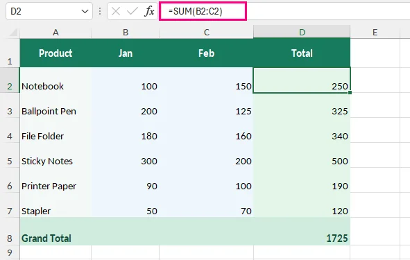
- Observe a Barra de Fórmulas acima da planilha para ver a fórmula.
Por exemplo, suponha que B2 e C2 contenham 100 e 150, respectivamente. A célula D2 usa a fórmula =SUM(B2:C2) para calcular o resultado 250. Quando você seleciona D2, a fórmula aparece na Barra de Fórmulas.
Opção 2: Usando o Modo de Edição
Para inspecionar a fórmula e suas células referenciadas diretamente na planilha:
Clique duas vezes na célula da fórmula ou pressione F2 no Windows.
O Excel exibe a fórmula dentro da célula e destaca suas referências.
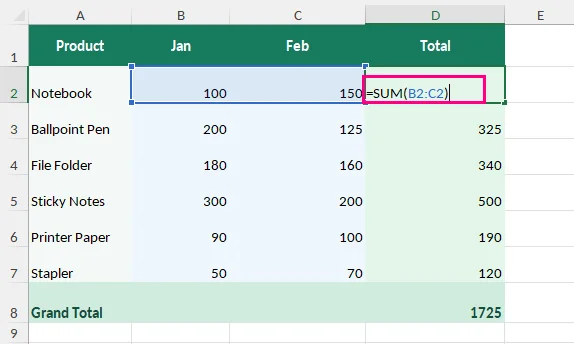
Pressione Esc para sair sem fazer alterações.
Dica: Se a Barra de Fórmulas estiver oculta, ative-a em:
Exibir > Mostrar > Barra de Fórmulas.
Mostrar todas as fórmulas em uma planilha do Excel
Ao revisar grandes modelos financeiros ou modelos de relatórios com muitos cálculos, verificar células uma a uma pode ser demorado. O Excel oferece opções integradas para exibir todas as fórmulas simultaneamente.
Opção 1: Usando o botão Mostrar Fórmulas
Abra a planilha que você deseja inspecionar.
Acesse Fórmulas > Mostrar Fórmulas no grupo Auditoria de Fórmulas.
O Excel exibe fórmulas no lugar de seus resultados calculados.
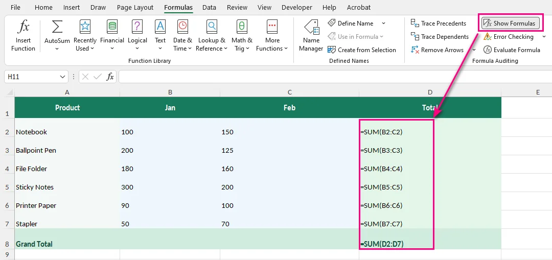
Dica: Você pode clicar em Mostrar Fórmulas novamente para retornar à visualização normal.
Opção 2: Usando um atalho de teclado
Pressione Ctrl + ` (a tecla de acento grave, geralmente localizada abaixo de Esc) no Windows para alternar entre fórmulas e valores calculados.
Observação: Esse recurso se aplica à planilha ativa e altera apenas a forma como as fórmulas são exibidas. Os cálculos subjacentes permanecem inalterados.
Se você precisar de uma cópia estática dos resultados, pode remover fórmulas no Excel mantendo os valores calculados.
Localizar células que contêm fórmulas no Excel
Se você não quiser exibir todas as fórmulas, mas precisar localizar células de fórmula rapidamente, use o recurso Ir Para Especial do Excel. Esse método é útil quando você precisa revisar fórmulas antes de editar, copiar ou converter dados de planilhas.
Selecione a planilha ou o intervalo que deseja pesquisar.
Acesse Página Inicial > Localizar e Selecionar > Ir Para Especial.
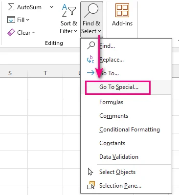
Selecione Fórmulas.
Clique em OK.
O Excel destaca as células que contêm fórmulas. Você também pode usar as opções em Fórmulas na caixa de diálogo Ir Para Especial para selecionar fórmulas com base em seus tipos de resultado. Para obter mais detalhes, consulte o guia da Microsoft sobre localizar células que contêm fórmulas.
Exibir fórmulas e resultados lado a lado
Se você precisar comparar fórmulas com seus resultados calculados, use a função FORMULATEXT. Ela exibe a fórmula de uma célula como texto em outra, sem afetar o cálculo original.
Por exemplo, suponha que a célula D2 exiba 250, calculado usando a fórmula =SUM(B2:C2).
Para exibir a fórmula ao lado de seu resultado:
Selecione uma célula vazia ao lado dela, como E2.
Insira a seguinte fórmula:
=FORMULATEXT(D2)Pressione Enter. A célula E2 exibe =SUM(B2:C2), enquanto D2 continua mostrando 250.
Arraste a alça de preenchimento para baixo para visualizar fórmulas de linhas adicionais.
O resultado é semelhante a este:
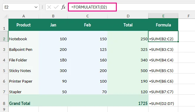
Isso é particularmente útil para verificar cálculos financeiros, revisar relatórios ou documentar fórmulas de planilhas.
Observação: De acordo com a documentação de FORMULATEXT da Microsoft, a função retorna #N/A se a célula referenciada não contiver uma fórmula, se a fórmula exceder 8.192 caracteres, se a fórmula não puder ser exibida devido à proteção da planilha ou se a pasta de trabalho externa referenciada estiver fechada.
Para deixar células em branco quando FORMULATEXT retornar um erro, use:
=IFERROR(FORMULATEXT(D2),"")
Como IFERROR captura todos os erros, não apenas #N/A, use esta opção somente quando um resultado em branco for preferível a ver uma mensagem de erro.
Por que não consigo ver fórmulas no Excel?
Se as fórmulas não forem exibidas como esperado, verifique estes problemas comuns:
- A Barra de Fórmulas está ausente: Acesse Exibir > Mostrar > Barra de Fórmulas para ativá-la.
- As fórmulas estão ocultas: A planilha pode estar protegida, impedindo que fórmulas ocultas apareçam na Barra de Fórmulas. Se você tiver permissão, acesse Revisão > Desproteger Planilha. Para manter as fórmulas visíveis quando a planilha for protegida novamente, selecione as células afetadas, abra Formatar Células > Proteção e desmarque a caixa de seleção Oculto.
- A fórmula aparece como texto em vez de um resultado: Primeiro, verifique se Mostrar Fórmulas está habilitado na guia Fórmulas. Se apenas algumas células exibirem fórmulas como texto, verifique se elas estão formatadas como Texto ou contêm um apóstrofo inicial. Altere o formato da célula para Geral, se necessário, remova qualquer apóstrofo inicial não intencional e insira a fórmula novamente pressionando F2 e depois Enter.
- FORMULATEXT retorna #N/A: Verifique se a célula referenciada contém uma fórmula. Referências a células em pastas de trabalho externas fechadas também podem causar esse erro.
Avançado: extrair fórmulas do Excel programaticamente com Python
Para desenvolvedores ou usuários que trabalham com vários arquivos do Excel, inspecionar manualmente fórmulas em planilhas pode ser demorado. O Python pode automatizar esse processo extraindo expressões de fórmulas e endereços de células de várias pastas de trabalho sem abrir manualmente cada arquivo.
O exemplo a seguir usa Free Spire.XLS for Python para extrair fórmulas em várias pastas de trabalho do Excel e salvá-las em um arquivo de texto. O Microsoft Excel não precisa estar instalado.
Etapa 1: Instalar o Free Spire.XLS
Execute o seguinte comando pip no terminal:
pip install spire.xls.free
Etapa 2: Extrair fórmulas de várias pastas de trabalho do Excel
Crie uma pasta chamada Excel Files e coloque nela as pastas de trabalho .xlsx que deseja processar.
O script a seguir examina cada pasta de trabalho, identifica células que contêm fórmulas e exporta seus locais e expressões para um arquivo de texto.
from pathlib import Path
from spire.xls import Workbook

# Input folder and output file
input_dir = Path("Excel Files")
output_file = Path("Extracted Formulas.txt")

# Check the input folder
if not input_dir.is_dir():
    raise FileNotFoundError(f"Input folder not found: {input_dir}")

# Get all Excel files in the folder
excel_files = sorted(
    file for file in input_dir.glob("*.xlsx")
    if file.is_file() and not file.name.startswith("~{BODY_CONTENT}quot;)
)

if not excel_files:
    raise FileNotFoundError(f"No XLSX files found in: {input_dir}")

formula_count = 0

# Extract formulas from all workbooks
with output_file.open("w", encoding="utf-8") as output:
    for input_file in excel_files:

        # Load the Excel workbook
        workbook = Workbook()
        try:
            workbook.LoadFromFile(str(input_file))

            # Loop through all worksheets
            for i in range(workbook.Worksheets.Count):
                sheet = workbook.Worksheets[i]

                # Get the used range
                used_range = sheet.AllocatedRange

                # Find and extract formulas
                for cell in used_range:
                    if cell.HasFormula:
                        cell_address = cell.RangeAddressLocal.replace("{BODY_CONTENT}quot;, "")
                        formula = cell.Formula

                        # Write formula information to the text file
                        output.write(f"{input_file.name} | {sheet.Name}!{cell_address}: {formula}\n")
                        formula_count += 1
        finally:
            workbook.Dispose()
Etapa 3: Verificar as fórmulas extraídas
Após executar o script, abra Extracted Formulas.txt. A saída será semelhante a esta:
Budget.xlsx | Forecast!E2: =IF(D2>1000,D2*0.1,0)
Sales Report.xlsx | Summary!D2: =SUM(B2:C2)
Sales Report.xlsx | Summary!D3: =SUM(B3:C3)
Cada linha identifica a pasta de trabalho de origem, a planilha, o local da célula e a fórmula, facilitando a pesquisa, a revisão ou a documentação de cálculos em vários arquivos.
Observação: O script lê expressões de fórmulas sem modificar as pastas de trabalho originais. Ele não recalcula fórmulas explicitamente. O Free Spire.XLS tem limites de planilhas e linhas para arquivos .xls mais antigos, mas esses limites não se aplicam a arquivos .xlsx.
Conclusão
Para uma fórmula, use a Barra de Fórmulas ou o Modo de Edição. Para exibir fórmulas em uma planilha inteira, use Mostrar Fórmulas. Para localizar células de fórmula, escolha Ir Para Especial; para comparar expressões e resultados, use FORMULATEXT. Se você precisar de expressões de fórmulas de muitas pastas de trabalho .xlsx, o método com Python pode automatizar a extração.
Perguntas frequentes
Posso mostrar fórmulas e valores ao mesmo tempo no Excel?
Sim. Você pode mostrar fórmulas e valores juntos usando a função FORMULATEXT. Por exemplo, se D2 contém uma fórmula, insira =FORMULATEXT(D2) em outra célula para exibir a fórmula enquanto mantém o valor calculado visível.
Como faço para ver fórmulas em vez de valores no Excel?
Selecione uma célula de fórmula e verifique a Barra de Fórmulas, ou habilite Mostrar Fórmulas na guia Fórmulas para exibir todas as fórmulas na planilha.
Por que o Excel está mostrando fórmulas em vez de resultados?
Se fórmulas aparecerem em toda a planilha, Mostrar Fórmulas pode estar habilitado. Pressione Ctrl + ` ou desative Fórmulas > Mostrar Fórmulas. Se apenas algumas células exibirem fórmulas como texto, verifique se elas estão formatadas como Texto ou contêm um apóstrofo inicial.
Posso extrair fórmulas do Excel sem abrir o Microsoft Excel?
Sim. Bibliotecas Python como o Free Spire.XLS podem carregar pastas de trabalho do Excel e extrair fórmulas sem iniciar o Microsoft Excel.
Tutoriais relacionados do Excel
엑셀에서 수식 보는 방법 (수식 표시, 찾기, 추출하기)
Excel은 일반적으로 수식 자체가 아니라 수식 결과를 표시합니다. 이렇게 하면 워크시트가 깔끔하고 읽기 쉬워지지만, 계산을 확인하거나 오류를 해결하거나 익숙하지 않은 통합 문서의 작동 방식을 이해해야 할 때 불편할 수 있습니다.
Excel에서 수식을 보는 방법은 여러 가지가 있습니다. 단일 셀을 검사하거나, 전체 워크시트를 검토하거나, 수식과 결과를 비교하거나, 여러 워크시트 또는 통합 문서에서 수식을 일괄 추출하려는 경우 등 상황에 따라 적합한 방법이 다릅니다. 아래 표가 올바른 방법을 선택하는 데 도움이 됩니다.
| 필요한 작업 | 최적의 방법 |
|---|---|
| 셀의 수식 보기 | 수식 입력줄 또는 편집 모드 |
| 워크시트의 모든 수식 표시 | 수식 표시 또는 Ctrl + ` |
| 수식이 포함된 셀 찾기 | 이동 옵션 |
| 수식과 결과를 나란히 보기 | FORMULATEXT 함수 |
| 여러 워크시트 또는 통합 문서에서 수식 추출 | Python 자동화 |
Excel에서 수식을 언제 확인해야 할까요?
수식 보기는 다음과 같은 경우에 특히 유용합니다:
- 재무 스프레드시트 감사
- 계산 오류 디버깅
- 다른 사용자가 만든 수식 검토
- 복사한 수식이 올바른 셀을 참조하는지 확인
- 규정 준수 검토를 위한 스프레드시트 준비
단일 셀의 수식 보기
특정 셀의 값이 어떻게 계산되었는지 확인하려면 워크시트를 변경하지 않고 수식 입력줄이나 편집 모드에서 해당 수식을 직접 볼 수 있습니다.
옵션 1: 수식 입력줄 사용
- 수식이 포함된 셀을 선택합니다.
- 워크시트 위의 수식 입력줄에서 수식을 확인합니다.
예를 들어 B2와 C2에 각각 100과 150이 포함되어 있다고 가정합니다. D2 셀은 =SUM(B2:C2) 수식을 사용하여 결과 250을 계산합니다. D2를 선택하면 수식 입력줄에 수식이 나타납니다.
옵션 2: 편집 모드 사용
워크시트에서 수식과 참조된 셀을 직접 검사하려면:
수식 셀을 두 번 클릭하거나 Windows에서 F2를 누릅니다.
Excel은 셀 안에 수식을 표시하고 참조를 강조 표시합니다.
변경하지 않고 나가려면 Esc를 누릅니다.
팁: 수식 입력줄이 숨겨져 있으면 다음에서 활성화하세요:
보기 > 표시 > 수식 입력줄.
Excel 워크시트의 모든 수식 표시
많은 계산이 포함된 대규모 재무 모델이나 보고 템플릿을 검토할 때 셀을 하나씩 확인하는 것은 시간이 많이 걸릴 수 있습니다. Excel은 모든 수식을 동시에 표시할 수 있는 기본 제공 옵션을 제공합니다.
옵션 1: 수식 표시 버튼 사용
검사할 워크시트를 엽니다.
수식 감사 그룹에서 수식 > 수식 표시로 이동합니다.
Excel은 계산된 결과 대신 수식을 표시합니다.
팁: 수식 표시를 다시 클릭하여 일반 보기로 돌아갈 수 있습니다.
옵션 2: 키보드 단축키 사용
Windows에서 Ctrl + `(일반적으로 Esc 아래에 있는 억음 부호 키)를 눌러 수식과 계산된 값 사이를 전환합니다.
참고: 이 기능은 활성 워크시트에 적용되며 수식이 표시되는 방식만 변경합니다. 기본 계산은 변경되지 않습니다.
대신 결과의 정적 복사본이 필요하면 계산된 값을 유지하면서 Excel에서 수식을 제거할 수 있습니다.
Excel에서 수식이 포함된 셀 찾기
모든 수식을 표시하고 싶지는 않지만 수식 셀을 빠르게 찾아야 하는 경우 Excel의 이동 옵션 기능을 사용하세요. 이 방법은 스프레드시트 데이터를 편집, 복사 또는 변환하기 전에 수식을 검토해야 할 때 유용합니다.
검색할 워크시트 또는 범위를 선택합니다.
홈 > 찾기 및 선택 > 이동 옵션으로 이동합니다.
수식을 선택합니다.
확인을 클릭합니다.
Excel은 수식이 포함된 셀을 강조 표시합니다. 이동 옵션 대화 상자의 수식 아래 옵션을 사용하여 결과 유형에 따라 수식을 선택할 수도 있습니다. 자세한 내용은 수식이 포함된 셀 찾기에 대한 Microsoft 가이드를 참조하세요.
수식과 결과를 나란히 보기
수식과 계산된 결과를 비교해야 하는 경우 FORMULATEXT 함수를 사용하세요. 이 함수는 원래 계산에 영향을 주지 않으면서 한 셀의 수식을 다른 셀에 텍스트로 표시합니다.
예를 들어 D2 셀에 =SUM(B2:C2) 수식으로 계산된 250이 표시된다고 가정합니다.
결과 옆에 수식을 표시하려면:
그 옆의 빈 셀(예: E2)을 선택합니다.
다음 수식을 입력합니다:
=FORMULATEXT(D2)Enter를 누릅니다. E2 셀에는 =SUM(B2:C2)가 표시되고 D2는 계속 250을 표시합니다.
채우기 핸들을 아래로 끌어 추가 행의 수식을 확인합니다.
결과는 다음과 같습니다:
이는 재무 계산을 확인하거나, 보고서를 검토하거나, 스프레드시트 수식을 문서화할 때 특히 유용합니다.
참고: Microsoft의 FORMULATEXT 문서에 따르면 참조된 셀에 수식이 없거나, 수식이 8,192자를 초과하거나, 워크시트 보호로 인해 수식을 표시할 수 없거나, 참조된 외부 통합 문서가 닫혀 있으면 이 함수는 #N/A를 반환합니다.
FORMULATEXT에서 오류가 반환될 때 셀을 비워 두려면 다음을 사용하세요:
=IFERROR(FORMULATEXT(D2),"")
IFERROR는 #N/A뿐만 아니라 모든 오류를 포착하므로 오류 메시지를 보는 것보다 빈 결과가 더 나은 경우에만 이 옵션을 사용하세요.
Excel에서 수식이 보이지 않는 이유는 무엇인가요?
수식이 예상대로 표시되지 않으면 다음과 같은 일반적인 문제를 확인하세요:
- 수식 입력줄이 없음: 보기 > 표시 > 수식 입력줄로 이동하여 활성화합니다.
- 수식이 숨겨져 있음: 워크시트가 보호되어 숨겨진 수식이 수식 입력줄에 나타나지 않을 수 있습니다. 권한이 있으면 검토 > 시트 보호 해제로 이동합니다. 시트를 다시 보호할 때도 수식이 표시되도록 하려면 영향을 받는 셀을 선택하고, 셀 서식 > 보호를 열고 숨김 확인란을 선택 취소합니다.
- 수식이 결과 대신 텍스트로 표시됨: 먼저 수식 탭에서 수식 표시가 활성화되어 있는지 확인합니다. 특정 셀만 수식을 텍스트로 표시하는 경우 텍스트로 서식이 지정되었거나 앞에 아포스트로피가 있는지 확인합니다. 필요한 경우 셀 서식을 일반으로 변경하고, 의도하지 않은 앞의 아포스트로피를 제거한 다음 F2를 누르고 Enter를 눌러 수식을 다시 입력합니다.
- FORMULATEXT가 #N/A를 반환함: 참조된 셀에 수식이 있는지 확인합니다. 닫힌 외부 통합 문서의 셀을 참조하는 경우에도 이 오류가 발생할 수 있습니다.
고급: Python으로 Excel 수식을 프로그래밍 방식으로 추출
여러 Excel 파일로 작업하는 개발자나 사용자의 경우 여러 워크시트의 수식을 수동으로 검사하는 것은 시간이 많이 걸릴 수 있습니다. Python은 각 파일을 수동으로 열지 않고도 여러 통합 문서에서 수식 표현식과 셀 주소를 추출하여 이 프로세스를 자동화할 수 있습니다.
다음 예제에서는 Free Spire.XLS for Python을 사용하여 여러 Excel 통합 문서에서 수식 추출하고 텍스트 파일에 저장합니다. Microsoft Excel을 설치할 필요가 없습니다.
1단계: Free Spire.XLS 설치
터미널에서 다음 pip 명령을 실행합니다:
pip install spire.xls.free
2단계: 여러 Excel 통합 문서에서 수식 추출
Excel Files라는 폴더를 만들고 처리할 .xlsx 통합 문서를 그 안에 넣습니다.
다음 스크립트는 각 통합 문서를 검사하여 수식이 포함된 셀을 식별하고 해당 위치와 표현식을 텍스트 파일로 내보냅니다.
from pathlib import Path
from spire.xls import Workbook

# Input folder and output file
input_dir = Path("Excel Files")
output_file = Path("Extracted Formulas.txt")

# Check the input folder
if not input_dir.is_dir():
    raise FileNotFoundError(f"Input folder not found: {input_dir}")

# Get all Excel files in the folder
excel_files = sorted(
    file for file in input_dir.glob("*.xlsx")
    if file.is_file() and not file.name.startswith("~{BODY_CONTENT}quot;)
)

if not excel_files:
    raise FileNotFoundError(f"No XLSX files found in: {input_dir}")

formula_count = 0

# Extract formulas from all workbooks
with output_file.open("w", encoding="utf-8") as output:
    for input_file in excel_files:

        # Load the Excel workbook
        workbook = Workbook()
        try:
            workbook.LoadFromFile(str(input_file))

            # Loop through all worksheets
            for i in range(workbook.Worksheets.Count):
                sheet = workbook.Worksheets[i]

                # Get the used range
                used_range = sheet.AllocatedRange

                # Find and extract formulas
                for cell in used_range:
                    if cell.HasFormula:
                        cell_address = cell.RangeAddressLocal.replace("{BODY_CONTENT}quot;, "")
                        formula = cell.Formula

                        # Write formula information to the text file
                        output.write(f"{input_file.name} | {sheet.Name}!{cell_address}: {formula}\n")
                        formula_count += 1
        finally:
            workbook.Dispose()
3단계: 추출된 수식 확인
스크립트를 실행한 후 Extracted Formulas.txt를 엽니다. 출력은 다음과 유사합니다:
Budget.xlsx | Forecast!E2: =IF(D2>1000,D2*0.1,0)
Sales Report.xlsx | Summary!D2: =SUM(B2:C2)
Sales Report.xlsx | Summary!D3: =SUM(B3:C3)
각 줄은 원본 통합 문서, 워크시트, 셀 위치 및 수식을 식별하므로 여러 파일에서 계산을 더 쉽게 검색, 검토 또는 문서화할 수 있습니다.
참고: 이 스크립트는 원본 통합 문서를 수정하지 않고 수식 표현식을 읽습니다. 수식을 명시적으로 다시 계산하지는 않습니다. Free Spire.XLS는 이전 .xls 파일에 대해 워크시트 및 행 제한이 있지만 이러한 제한은 .xlsx 파일에는 적용되지 않습니다.
마무리
수식 하나를 보려면 수식 입력줄 또는 편집 모드를 사용하세요. 워크시트 전체에서 수식을 표시하려면 수식 표시를 사용하세요. 수식 셀을 찾으려면 이동 옵션을 선택하고, 표현식과 결과를 비교하려면 FORMULATEXT를 사용하세요. 많은 .xlsx 통합 문서에서 수식 표현식이 필요하면 Python 방법으로 추출을 자동화할 수 있습니다.
자주 묻는 질문
Excel에서 수식과 값을 동시에 표시할 수 있나요?
예. FORMULATEXT 함수를 사용하여 수식과 값을 함께 표시할 수 있습니다. 예를 들어 D2에 수식이 있으면 다른 셀에 =FORMULATEXT(D2)를 입력하여 계산된 값을 계속 표시하면서 수식을 표시할 수 있습니다.
Excel에서 값 대신 수식을 보려면 어떻게 하나요?
수식 셀을 선택하고 수식 입력줄을 확인하거나 수식 탭에서 수식 표시를 활성화하여 워크시트의 모든 수식을 표시합니다.
Excel에서 결과 대신 수식이 표시되는 이유는 무엇인가요?
워크시트 전체에 수식이 나타나면 수식 표시가 활성화되어 있을 수 있습니다. Ctrl + `를 누르거나 수식 > 수식 표시를 비활성화하세요. 특정 셀만 수식을 텍스트로 표시하는 경우 텍스트로 서식이 지정되었거나 앞에 아포스트로피가 있는지 확인하세요.
Microsoft Excel을 열지 않고 Excel 수식을 추출할 수 있나요?
예. Free Spire.XLS와 같은 Python 라이브러리는 Microsoft Excel을 실행하지 않고도 Excel 통합 문서를 로드하고 수식을 추출할 수 있습니다.
관련 Excel 튜토리얼
Come visualizzare le formule in Excel (mostrare, trovare ed estrarre formule)
Indice
- Quando dovresti visualizzare le formule in Excel?
- Visualizzare una formula in una singola cella
- Mostrare tutte le formule in un foglio di lavoro Excel
- Trovare le celle che contengono formule in Excel
- Visualizzare formule e risultati affiancati
- Perché non riesco a vedere le formule in Excel?
- Avanzato: estrarre formule Excel a livello di codice con Python
- Conclusione
- Domande frequenti
- Tutorial Excel correlati
Excel normalmente mostra i risultati delle formule anziché le formule stesse. Questo rende i fogli di lavoro puliti e facili da leggere, ma può essere scomodo quando devi controllare i calcoli, risolvere errori o capire come funziona una cartella di lavoro che non conosci.
Esistono diversi modi per visualizzare le formule in Excel, che tu voglia esaminare una singola cella, rivedere un intero foglio di lavoro, confrontare le formule con i relativi risultati o estrarre formule da più fogli di lavoro o cartelle di lavoro in blocco. La tabella seguente ti aiuterà a scegliere il metodo giusto.
| Cosa ti serve | Metodo migliore |
|---|---|
| Visualizzare una formula in una cella | Barra della formula o modalità di modifica |
| Mostrare tutte le formule in un foglio di lavoro | Mostra formule o Ctrl + ` |
| Trovare le celle che contengono formule | Vai a speciale |
| Visualizzare le formule accanto ai relativi risultati | Funzione FORMULATEXT |
| Estrarre formule da più fogli di lavoro o cartelle di lavoro | Automazione con Python |
Quando dovresti visualizzare le formule in Excel?
Visualizzare le formule è particolarmente utile quando:
- Revisione di fogli di calcolo finanziari
- Debug di errori di calcolo
- Revisione di formule create da altri utenti
- Controllo che le formule copiate facciano riferimento alle celle corrette
- Preparazione di fogli di calcolo per revisioni di conformità
Visualizzare una formula in una singola cella
Se vuoi controllare come è stato calcolato un valore in una cella specifica, puoi visualizzare la relativa formula direttamente nella barra della formula o in modalità di modifica senza modificare il foglio di lavoro.
Opzione 1: usare la barra della formula
- Seleziona la cella che contiene la formula.
- Guarda la Barra della formula sopra il foglio di lavoro per vedere la formula.
Ad esempio, supponi che B2 e C2 contengano rispettivamente 100 e 150. La cella D2 usa la formula =SUM(B2:C2) per calcolare il risultato 250. Quando selezioni D2, la formula viene visualizzata nella barra della formula.
Opzione 2: usare la modalità di modifica
Per esaminare la formula e le celle a cui fa riferimento direttamente nel foglio di lavoro:
Fai doppio clic sulla cella della formula o premi F2 in Windows.
Excel visualizza la formula all'interno della cella ed evidenzia i relativi riferimenti.
Premi Esc per uscire senza apportare modifiche.
Suggerimento: Se la barra della formula è nascosta, abilitala in:
Visualizza > Mostra > Barra della formula.
Mostrare tutte le formule in un foglio di lavoro Excel
Quando si esaminano modelli finanziari di grandi dimensioni o modelli di report con molti calcoli, controllare le celle una per una può richiedere molto tempo. Excel fornisce opzioni integrate per visualizzare tutte le formule contemporaneamente.
Opzione 1: usare il pulsante Mostra formule
Apri il foglio di lavoro che vuoi esaminare.
Vai a Formule > Mostra formule nel gruppo Controllo formule.
Excel visualizza le formule al posto dei risultati calcolati.
Suggerimento: Puoi fare di nuovo clic su Mostra formule per tornare alla visualizzazione normale.
Opzione 2: usare una scorciatoia da tastiera
Premi Ctrl + ` (il tasto accento grave, di solito si trova sotto Esc) in Windows per passare da formule a valori calcolati e viceversa.
Nota: questa funzione si applica al foglio di lavoro attivo e cambia solo il modo in cui vengono visualizzate le formule. I calcoli sottostanti rimangono invariati.
Se invece ti serve una copia statica dei risultati, puoi rimuovere le formule in Excel mantenendo i valori calcolati.
Trovare le celle che contengono formule in Excel
Se non vuoi visualizzare tutte le formule ma devi individuare rapidamente le celle con formule, usa la funzione Vai a speciale di Excel. Questo metodo è utile quando devi rivedere le formule prima di modificare, copiare o convertire i dati di un foglio di calcolo.
Seleziona il foglio di lavoro o l'intervallo che vuoi cercare.
Vai a Home > Trova e seleziona > Vai a speciale.
Seleziona Formule.
Fai clic su OK.
Excel evidenzia le celle che contengono formule. Puoi anche usare le opzioni sotto Formule nella finestra di dialogo Vai a speciale per selezionare le formule in base ai relativi tipi di risultato. Per maggiori dettagli, consulta la guida di Microsoft su trovare le celle che contengono formule.
Visualizzare formule e risultati affiancati
Se devi confrontare le formule con i relativi risultati calcolati, usa la funzione FORMULATEXT. Visualizza la formula di una cella come testo in un'altra cella, senza modificare il calcolo originale.
Ad esempio, supponi che la cella D2 mostri 250, calcolato con la formula =SUM(B2:C2).
Per visualizzare la formula accanto al relativo risultato:
Seleziona una cella vuota accanto, ad esempio E2.
Immetti la formula seguente:
=FORMULATEXT(D2)Premi Invio. La cella E2 visualizza =SUM(B2:C2), mentre D2 continua a mostrare 250.
Trascina il quadratino di riempimento verso il basso per visualizzare le formule per altre righe.
Il risultato è simile al seguente:
Questo è particolarmente utile per controllare calcoli finanziari, rivedere report o documentare le formule di un foglio di calcolo.
Nota: secondo la documentazione di Microsoft su FORMULATEXT, la funzione restituisce #N/A se la cella a cui si fa riferimento non contiene una formula, se la formula supera 8.192 caratteri, se la formula non può essere visualizzata a causa della protezione del foglio di lavoro o se la cartella di lavoro esterna a cui si fa riferimento è chiusa.
Per lasciare vuote le celle quando FORMULATEXT restituisce un errore, usa:
=IFERROR(FORMULATEXT(D2),"")
Poiché IFERROR intercetta tutti gli errori, non solo #N/A, usa questa opzione solo quando un risultato vuoto è preferibile alla visualizzazione di un messaggio di errore.
Perché non riesco a vedere le formule in Excel?
Se le formule non vengono visualizzate come previsto, controlla questi problemi comuni:
- La barra della formula è mancante: Vai a Visualizza > Mostra > Barra della formula per abilitarla.
- Le formule sono nascoste: Il foglio di lavoro potrebbe essere protetto, impedendo la visualizzazione delle formule nascoste nella barra della formula. Se disponi delle autorizzazioni necessarie, vai a Revisione > Rimuovi protezione foglio. Per mantenere visibili le formule quando il foglio viene protetto di nuovo, seleziona le celle interessate, apri Formato celle > Protezione e deseleziona la casella Nascoste.
- La formula viene visualizzata come testo invece che come risultato: Innanzitutto, controlla se Mostra formule è abilitato nella scheda Formule. Se solo alcune celle visualizzano le formule come testo, controlla se sono formattate come Testo o contengono un apostrofo iniziale. Se necessario, cambia il formato della cella in Generale, rimuovi eventuali apostrofi iniziali indesiderati e reimmetti la formula premendo F2 e poi Invio.
- FORMULATEXT restituisce #N/A: Controlla se la cella a cui si fa riferimento contiene una formula. Anche i riferimenti a celle in cartelle di lavoro esterne chiuse possono causare questo errore.
Avanzato: estrarre formule Excel a livello di codice con Python
Per gli sviluppatori o gli utenti che lavorano con più file Excel, esaminare manualmente le formule nei vari fogli di lavoro può richiedere molto tempo. Python può automatizzare questo processo estraendo espressioni di formule e indirizzi di celle da più cartelle di lavoro senza aprire manualmente ogni file.
L'esempio seguente usa Free Spire.XLS for Python per estrarre formule in più cartelle di lavoro Excel e salvarle in un file di testo. Non è necessario installare Microsoft Excel.
Passaggio 1: installare Free Spire.XLS
Esegui il comando pip seguente nel terminale:
pip install spire.xls.free
Passaggio 2: estrarre formule da più cartelle di lavoro Excel
Crea una cartella denominata Excel Files e inserisci al suo interno le cartelle di lavoro .xlsx che vuoi elaborare.
Lo script seguente analizza ogni cartella di lavoro, identifica le celle che contengono formule ed esporta le relative posizioni ed espressioni in un file di testo.
from pathlib import Path
from spire.xls import Workbook

# Input folder and output file
input_dir = Path("Excel Files")
output_file = Path("Extracted Formulas.txt")

# Check the input folder
if not input_dir.is_dir():
    raise FileNotFoundError(f"Input folder not found: {input_dir}")

# Get all Excel files in the folder
excel_files = sorted(
    file for file in input_dir.glob("*.xlsx")
    if file.is_file() and not file.name.startswith("~{BODY_CONTENT}quot;)
)

if not excel_files:
    raise FileNotFoundError(f"No XLSX files found in: {input_dir}")

formula_count = 0

# Extract formulas from all workbooks
with output_file.open("w", encoding="utf-8") as output:
    for input_file in excel_files:

        # Load the Excel workbook
        workbook = Workbook()
        try:
            workbook.LoadFromFile(str(input_file))

            # Loop through all worksheets
            for i in range(workbook.Worksheets.Count):
                sheet = workbook.Worksheets[i]

                # Get the used range
                used_range = sheet.AllocatedRange

                # Find and extract formulas
                for cell in used_range:
                    if cell.HasFormula:
                        cell_address = cell.RangeAddressLocal.replace("{BODY_CONTENT}quot;, "")
                        formula = cell.Formula

                        # Write formula information to the text file
                        output.write(f"{input_file.name} | {sheet.Name}!{cell_address}: {formula}\n")
                        formula_count += 1
        finally:
            workbook.Dispose()
Passaggio 3: controllare le formule estratte
Dopo aver eseguito lo script, apri Extracted Formulas.txt. L'output sarà simile al seguente:
Budget.xlsx | Forecast!E2: =IF(D2>1000,D2*0.1,0)
Sales Report.xlsx | Summary!D2: =SUM(B2:C2)
Sales Report.xlsx | Summary!D3: =SUM(B3:C3)
Ogni riga identifica la cartella di lavoro di origine, il foglio di lavoro, la posizione della cella e la formula, rendendo più semplice cercare, rivedere o documentare i calcoli in più file.
Nota: lo script legge le espressioni delle formule senza modificare le cartelle di lavoro originali. Non ricalcola esplicitamente le formule. Free Spire.XLS ha limiti di fogli di lavoro e righe per i file .xls meno recenti, ma questi limiti non si applicano ai file .xlsx.
Conclusione
Per una singola formula, usa la barra della formula o la modalità di modifica. Per visualizzare le formule in tutto un foglio di lavoro, usa Mostra formule. Per individuare le celle con formule, scegli Vai a speciale; per confrontare espressioni e risultati, usa FORMULATEXT. Se hai bisogno delle espressioni di formula da molte cartelle di lavoro .xlsx, il metodo Python può automatizzare l'estrazione.
Domande frequenti
Posso mostrare formule e valori contemporaneamente in Excel?
Sì. Puoi mostrare formule e valori insieme usando la funzione FORMULATEXT. Ad esempio, se D2 contiene una formula, immetti =FORMULATEXT(D2) in un'altra cella per visualizzare la formula mantenendo visibile il valore calcolato.
Come posso vedere le formule invece dei valori in Excel?
Seleziona una cella con formula e controlla la barra della formula, oppure abilita Mostra formule dalla scheda Formule per visualizzare tutte le formule nel foglio di lavoro.
Perché Excel mostra le formule invece dei risultati?
Se le formule appaiono in tutto il foglio di lavoro, Mostra formule potrebbe essere abilitato. Premi Ctrl + ` o disabilita Formule > Mostra formule. Se solo alcune celle visualizzano le formule come testo, controlla se sono formattate come Testo o contengono un apostrofo iniziale.
Posso estrarre formule Excel senza aprire Microsoft Excel?
Sì. Librerie Python come Free Spire.XLS possono caricare cartelle di lavoro Excel ed estrarre formule senza avviare Microsoft Excel.
Tutorial Excel correlati
Comment afficher les formules dans Excel (afficher, trouver et extraire les formules)
Table des matières
- Quand devez-vous afficher les formules dans Excel ?
- Afficher une formule dans une seule cellule
- Afficher toutes les formules dans une feuille de calcul Excel
- Rechercher les cellules qui contiennent des formules dans Excel
- Afficher les formules et les résultats côte à côte
- Pourquoi ne puis-je pas voir les formules dans Excel ?
- Avancé : extraire des formules Excel par programmation avec Python
- Conclusion
- Questions fréquentes
- Tutoriels Excel associés
Excel affiche normalement les résultats des formules plutôt que les formules elles-mêmes. Cela rend les feuilles de calcul propres et faciles à lire, mais cela peut être gênant lorsque vous devez vérifier des calculs, résoudre des erreurs ou comprendre le fonctionnement d’un classeur inconnu.
Il existe plusieurs façons d’afficher les formules dans Excel, que vous souhaitiez examiner une seule cellule, passer en revue une feuille de calcul entière, comparer des formules avec leurs résultats ou extraire des formules de plusieurs feuilles de calcul ou classeurs en masse. Le tableau ci-dessous vous aidera à choisir la bonne méthode.
| Ce dont vous avez besoin | Meilleure méthode |
|---|---|
| Afficher une formule dans une cellule | Barre de formule ou mode Édition |
| Afficher toutes les formules dans une feuille de calcul | Afficher les formules ou Ctrl + ` |
| Rechercher les cellules qui contiennent des formules | Atteindre (Spécial) |
| Afficher les formules à côté de leurs résultats | Fonction FORMULATEXT |
| Extraire des formules de plusieurs feuilles de calcul ou classeurs | Automatisation Python |
Quand devez-vous afficher les formules dans Excel ?
L’affichage des formules est particulièrement utile lorsque :
- Vous auditez des feuilles de calcul financières
- Vous déboguez des erreurs de calcul
- Vous vérifiez des formules créées par d’autres utilisateurs
- Vous vérifiez si les formules copiées font référence aux bonnes cellules
- Vous préparez des feuilles de calcul pour des contrôles de conformité
Afficher une formule dans une seule cellule
Si vous souhaitez vérifier comment une valeur d’une cellule particulière a été calculée, vous pouvez afficher sa formule directement dans la barre de formule ou en mode Édition sans modifier la feuille de calcul.
Option 1 : utiliser la barre de formule
- Sélectionnez la cellule contenant la formule.
- Regardez la barre de formule au-dessus de la feuille de calcul pour voir la formule.
Par exemple, supposons que B2 et C2 contiennent respectivement 100 et 150. La cellule D2 utilise la formule =SUM(B2:C2) pour calculer le résultat 250. Lorsque vous sélectionnez D2, la formule apparaît dans la barre de formule.
Option 2 : utiliser le mode Édition
Pour examiner la formule et ses cellules référencées directement dans la feuille de calcul :
Double-cliquez sur la cellule de formule ou appuyez sur F2 sous Windows.
Excel affiche la formule dans la cellule et met en évidence ses références.
Appuyez sur Échap pour quitter sans effectuer de modifications.
Astuce : si la barre de formule est masquée, activez-la sous :
Affichage > Afficher > Barre de formule.
Afficher toutes les formules dans une feuille de calcul Excel
Lorsque vous examinez de grands modèles financiers ou des modèles de reporting comportant de nombreux calculs, la vérification cellule par cellule peut prendre du temps. Excel propose des options intégrées pour afficher toutes les formules simultanément.
Option 1 : utiliser le bouton Afficher les formules
Ouvrez la feuille de calcul que vous souhaitez examiner.
Accédez à Formules > Afficher les formules dans le groupe Audit des formules.
Excel affiche les formules à la place de leurs résultats calculés.
Astuce : vous pouvez cliquer à nouveau sur Afficher les formules pour revenir à la vue normale.
Option 2 : utiliser un raccourci clavier
Appuyez sur Ctrl + ` (la touche accent grave, généralement située sous Échap) sous Windows pour basculer entre les formules et les valeurs calculées.
Remarque : cette fonctionnalité s’applique à la feuille de calcul active et modifie uniquement la façon dont les formules sont affichées. Les calculs sous-jacents restent inchangés.
Si vous avez besoin d’une copie statique des résultats à la place, vous pouvez supprimer les formules dans Excel tout en conservant les valeurs calculées.
Rechercher les cellules qui contiennent des formules dans Excel
Si vous ne souhaitez pas afficher toutes les formules mais devez localiser rapidement les cellules de formule, utilisez la fonctionnalité Atteindre (Spécial) d’Excel. Cette méthode est utile lorsque vous devez vérifier des formules avant de modifier, copier ou convertir des données de feuille de calcul.
Sélectionnez la feuille de calcul ou la plage que vous souhaitez rechercher.
Accédez à Accueil > Rechercher et sélectionner > Atteindre (Spécial).
Sélectionnez Formules.
Cliquez sur OK.
Excel met en évidence les cellules contenant des formules. Vous pouvez également utiliser les options sous Formules dans la boîte de dialogue Atteindre (Spécial) pour sélectionner des formules en fonction de leurs types de résultat. Pour plus de détails, consultez le guide Microsoft sur la recherche des cellules qui contiennent des formules.
Afficher les formules et les résultats côte à côte
Si vous devez comparer des formules avec leurs résultats calculés, utilisez la fonction FORMULATEXT. Elle affiche la formule d’une cellule sous forme de texte dans une autre, sans affecter le calcul d’origine.
Par exemple, supposons que la cellule D2 affiche 250, calculé à l’aide de la formule =SUM(B2:C2).
Pour afficher la formule à côté de son résultat :
Sélectionnez une cellule vide à côté, par exemple E2.
Saisissez la formule suivante :
=FORMULATEXT(D2)Appuyez sur Entrée. La cellule E2 affiche =SUM(B2:C2), tandis que D2 continue d’afficher 250.
Faites glisser la poignée de recopie vers le bas pour afficher les formules des lignes supplémentaires.
Le résultat ressemble à ceci :
Cela est particulièrement utile pour vérifier des calculs financiers, examiner des rapports ou documenter des formules de feuille de calcul.
Remarque : selon la documentation Microsoft de FORMULATEXT, la fonction renvoie #N/A si la cellule référencée ne contient pas de formule, si la formule dépasse 8 192 caractères, si la formule ne peut pas être affichée en raison de la protection de la feuille de calcul ou si le classeur externe référencé est fermé.
Pour laisser des cellules vides lorsque FORMULATEXT renvoie une erreur, utilisez :
=IFERROR(FORMULATEXT(D2),"")
Étant donné qu’IFERROR intercepte toutes les erreurs, pas seulement #N/A, n’utilisez cette option que lorsqu’un résultat vide est préférable à l’affichage d’un message d’erreur.
Pourquoi ne puis-je pas voir les formules dans Excel ?
Si les formules ne s’affichent pas comme prévu, vérifiez ces problèmes courants :
- La barre de formule est absente : accédez à Affichage > Afficher > Barre de formule pour l’activer.
- Les formules sont masquées : la feuille de calcul peut être protégée, ce qui empêche les formules masquées d’apparaître dans la barre de formule. Si vous disposez des autorisations nécessaires, accédez à Révision > Ôter la protection de la feuille. Pour que les formules restent visibles lorsque la feuille est à nouveau protégée, sélectionnez les cellules concernées, ouvrez Format de cellule > Protection et décochez la case Masquée.
- La formule apparaît sous forme de texte au lieu d’un résultat : vérifiez d’abord si Afficher les formules est activé sous l’onglet Formules. Si seules certaines cellules affichent des formules sous forme de texte, vérifiez si elles sont mises au format Texte ou contiennent une apostrophe initiale. Modifiez le format de cellule en Général si nécessaire, supprimez toute apostrophe initiale involontaire, puis saisissez à nouveau la formule en appuyant sur F2 et ensuite sur Entrée.
- FORMULATEXT renvoie #N/A : vérifiez si la cellule référencée contient une formule. Les références à des cellules situées dans des classeurs externes fermés peuvent également provoquer cette erreur.
Avancé : extraire des formules Excel par programmation avec Python
Pour les développeurs ou les utilisateurs qui travaillent avec plusieurs fichiers Excel, l’inspection manuelle des formules dans les feuilles de calcul peut prendre du temps. Python peut automatiser ce processus en extrayant les expressions de formule et les adresses de cellule de plusieurs classeurs sans ouvrir manuellement chaque fichier.
L’exemple suivant utilise Free Spire.XLS for Python pour extraire des formules dans plusieurs classeurs Excel et les enregistrer dans un fichier texte. Microsoft Excel n’a pas besoin d’être installé.
Étape 1 : installer Free Spire.XLS
Exécutez la commande pip suivante dans votre terminal :
pip install spire.xls.free
Étape 2 : extraire les formules de plusieurs classeurs Excel
Créez un dossier nommé Excel Files et placez-y les classeurs .xlsx que vous souhaitez traiter.
Le script suivant analyse chaque classeur, identifie les cellules contenant des formules et exporte leurs emplacements et expressions dans un fichier texte.
from pathlib import Path
from spire.xls import Workbook

# Input folder and output file
input_dir = Path("Excel Files")
output_file = Path("Extracted Formulas.txt")

# Check the input folder
if not input_dir.is_dir():
    raise FileNotFoundError(f"Input folder not found: {input_dir}")

# Get all Excel files in the folder
excel_files = sorted(
    file for file in input_dir.glob("*.xlsx")
    if file.is_file() and not file.name.startswith("~{BODY_CONTENT}quot;)
)

if not excel_files:
    raise FileNotFoundError(f"No XLSX files found in: {input_dir}")

formula_count = 0

# Extract formulas from all workbooks
with output_file.open("w", encoding="utf-8") as output:
    for input_file in excel_files:

        # Load the Excel workbook
        workbook = Workbook()
        try:
            workbook.LoadFromFile(str(input_file))

            # Loop through all worksheets
            for i in range(workbook.Worksheets.Count):
                sheet = workbook.Worksheets[i]

                # Get the used range
                used_range = sheet.AllocatedRange

                # Find and extract formulas
                for cell in used_range:
                    if cell.HasFormula:
                        cell_address = cell.RangeAddressLocal.replace("{BODY_CONTENT}quot;, "")
                        formula = cell.Formula

                        # Write formula information to the text file
                        output.write(f"{input_file.name} | {sheet.Name}!{cell_address}: {formula}\n")
                        formula_count += 1
        finally:
            workbook.Dispose()
Étape 3 : vérifier les formules extraites
Après avoir exécuté le script, ouvrez Extracted Formulas.txt. La sortie ressemblera à ceci :
Budget.xlsx | Forecast!E2: =IF(D2>1000,D2*0.1,0)
Sales Report.xlsx | Summary!D2: =SUM(B2:C2)
Sales Report.xlsx | Summary!D3: =SUM(B3:C3)
Chaque ligne identifie le classeur source, la feuille de calcul, l’emplacement de la cellule et la formule, ce qui facilite la recherche, la vérification ou la documentation des calculs dans plusieurs fichiers.
Remarque : le script lit les expressions de formule sans modifier les classeurs d’origine. Il ne recalcule pas explicitement les formules. Free Spire.XLS a des limites de feuilles de calcul et de lignes pour les anciens fichiers .xls, mais ces limites ne s’appliquent pas aux fichiers .xlsx.
Conclusion
Pour une seule formule, utilisez la barre de formule ou le mode Édition. Pour afficher les formules dans une feuille de calcul, utilisez Afficher les formules. Pour localiser les cellules de formule, choisissez Atteindre (Spécial) ; pour comparer les expressions et les résultats, utilisez FORMULATEXT. Si vous avez besoin des expressions de formule de nombreux classeurs .xlsx, la méthode Python peut automatiser l’extraction.
Questions fréquentes
Puis-je afficher les formules et les valeurs en même temps dans Excel ?
Oui. Vous pouvez afficher les formules et les valeurs ensemble en utilisant la fonction FORMULATEXT. Par exemple, si D2 contient une formule, saisissez =FORMULATEXT(D2) dans une autre cellule pour afficher la formule tout en gardant la valeur calculée visible.
Comment voir les formules au lieu des valeurs dans Excel ?
Sélectionnez une cellule de formule et consultez la barre de formule, ou activez Afficher les formules dans l’onglet Formules pour afficher toutes les formules de la feuille de calcul.
Pourquoi Excel affiche-t-il des formules au lieu des résultats ?
Si des formules apparaissent dans toute la feuille de calcul, Afficher les formules peut être activé. Appuyez sur Ctrl + ` ou désactivez Formules > Afficher les formules. Si seules certaines cellules affichent des formules sous forme de texte, vérifiez si elles sont mises au format Texte ou contiennent une apostrophe initiale.
Puis-je extraire des formules Excel sans ouvrir Microsoft Excel ?
Oui. Des bibliothèques Python telles que Free Spire.XLS peuvent charger des classeurs Excel et extraire des formules sans lancer Microsoft Excel.
Tutoriels Excel associés
Cómo ver fórmulas en Excel (mostrar, encontrar y extraer fórmulas)
Tabla de contenido
- ¿Cuándo debería ver las fórmulas en Excel?
- Ver una fórmula en una sola celda
- Mostrar todas las fórmulas en una hoja de cálculo de Excel
- Buscar celdas que contengan fórmulas en Excel
- Ver fórmulas y resultados en paralelo
- ¿Por qué no puedo ver las fórmulas en Excel?
- Avanzado: Extraer fórmulas de Excel mediante programación con Python
- Conclusión
- Preguntas frecuentes
- Tutoriales de Excel relacionados
Normalmente, Excel muestra los resultados de las fórmulas en lugar de las fórmulas en sí. Esto hace que las hojas de cálculo sean limpias y fáciles de leer, pero puede resultar inconveniente cuando necesita comprobar cálculos, solucionar errores o entender cómo funciona un libro de trabajo desconocido.
Existen varias formas de ver fórmulas en Excel, ya sea que desee inspeccionar una sola celda, revisar toda una hoja de cálculo, comparar fórmulas con sus resultados o extraer fórmulas de varias hojas de cálculo o libros de trabajo en lote. La siguiente tabla le ayudará a elegir el método adecuado.
| Lo que necesita | Mejor método |
|---|---|
| Ver una fórmula en una celda | Barra de fórmulas o modo de edición |
| Mostrar todas las fórmulas en una hoja de cálculo | Mostrar fórmulas o Ctrl + ` |
| Buscar celdas que contengan fórmulas | Ir a Especial |
| Ver fórmulas junto con sus resultados | Función FORMULATEXT |
| Extraer fórmulas de varias hojas de cálculo o libros de trabajo | Automatización con Python |
¿Cuándo debería ver las fórmulas en Excel?
Ver las fórmulas resulta especialmente útil cuando:
- Audita hojas de cálculo financieras
- Depura errores de cálculo
- Revisa fórmulas creadas por otros usuarios
- Comprueba si las fórmulas copiadas hacen referencia a las celdas correctas
- Prepara hojas de cálculo para revisiones de cumplimiento
Ver una fórmula en una sola celda
Si desea comprobar cómo se calculó un valor en una celda concreta, puede ver su fórmula directamente en la barra de fórmulas o en el modo de edición sin modificar la hoja de cálculo.
Opción 1: Usar la barra de fórmulas
- Seleccione la celda que contiene la fórmula.
- Observe la barra de fórmulas situada encima de la hoja de cálculo para ver la fórmula.
Por ejemplo, suponga que B2 y C2 contienen 100 y 150, respectivamente. La celda D2 usa la fórmula =SUM(B2:C2) para calcular el resultado 250. Cuando selecciona D2, la fórmula aparece en la barra de fórmulas.
Opción 2: Usar el modo de edición
Para inspeccionar la fórmula y sus celdas referenciadas directamente en la hoja de cálculo:
Haga doble clic en la celda con la fórmula o pulse F2 en Windows.
Excel muestra la fórmula dentro de la celda y resalta sus referencias.
Pulse Esc para salir sin realizar cambios.
Consejo: Si la barra de fórmulas está oculta, actívela en:
Vista > Mostrar > Barra de fórmulas.
Mostrar todas las fórmulas en una hoja de cálculo de Excel
Al revisar grandes modelos financieros o plantillas de informes con muchos cálculos, comprobar las celdas una por una puede llevar mucho tiempo. Excel ofrece opciones integradas para mostrar todas las fórmulas simultáneamente.
Opción 1: Usar el botón Mostrar fórmulas
Abra la hoja de cálculo que desea inspeccionar.
Vaya a Fórmulas > Mostrar fórmulas en el grupo Auditoría de fórmulas.
Excel muestra las fórmulas en lugar de sus resultados calculados.
Consejo: Puede hacer clic de nuevo en Mostrar fórmulas para volver a la vista normal.
Opción 2: Usar un atajo de teclado
Pulse Ctrl + ` (la tecla de acento grave, normalmente situada debajo de Esc) en Windows para alternar entre fórmulas y valores calculados.
Nota: Esta función se aplica a la hoja de cálculo activa y solo cambia la forma en que se muestran las fórmulas. Los cálculos subyacentes permanecen sin cambios.
Si, en cambio, necesita una copia estática de los resultados, puede eliminar las fórmulas en Excel manteniendo los valores calculados.
Buscar celdas que contengan fórmulas en Excel
Si no desea mostrar todas las fórmulas, pero necesita localizar rápidamente las celdas con fórmulas, use la función Ir a Especial de Excel. Este método resulta útil cuando necesita revisar fórmulas antes de editar, copiar o convertir datos de una hoja de cálculo.
Seleccione la hoja de cálculo o el rango que desea buscar.
Vaya a Inicio > Buscar y seleccionar > Ir a Especial.
Seleccione Fórmulas.
Haga clic en Aceptar.
Excel resalta las celdas que contienen fórmulas. También puede usar las opciones que aparecen bajo Fórmulas en el cuadro de diálogo Ir a Especial para seleccionar fórmulas según sus tipos de resultado. Para obtener más detalles, consulte la guía de Microsoft sobre cómo encontrar celdas que contienen fórmulas.
Ver fórmulas y resultados en paralelo
Si necesita comparar fórmulas con sus resultados calculados, use la función FORMULATEXT. Muestra la fórmula de una celda como texto en otra, sin afectar el cálculo original.
Por ejemplo, suponga que la celda D2 muestra 250, calculado con la fórmula =SUM(B2:C2).
Para mostrar la fórmula junto a su resultado:
Seleccione una celda vacía junto a ella, como E2.
Introduzca la siguiente fórmula:
=FORMULATEXT(D2)Pulse Intro. La celda E2 muestra =SUM(B2:C2), mientras que D2 sigue mostrando 250.
Arrastre el controlador de relleno hacia abajo para ver las fórmulas de filas adicionales.
El resultado es similar a este:
Esto resulta especialmente útil para comprobar cálculos financieros, revisar informes o documentar fórmulas de hojas de cálculo.
Nota: Según la documentación de FORMULATEXT de Microsoft, la función devuelve #N/A si la celda a la que se hace referencia no contiene una fórmula, si la fórmula supera los 8.192 caracteres, si la fórmula no se puede mostrar debido a la protección de la hoja de cálculo o si el libro externo al que se hace referencia está cerrado.
Para dejar las celdas en blanco cuando FORMULATEXT devuelve un error, use:
=IFERROR(FORMULATEXT(D2),"")
Dado que IFERROR captura todos los errores, no solo #N/A, use esta opción solo cuando un resultado en blanco sea preferible a ver un mensaje de error.
¿Por qué no puedo ver las fórmulas en Excel?
Si las fórmulas no se muestran como espera, revise estos problemas comunes:
- Falta la barra de fórmulas: Vaya a Vista > Mostrar > Barra de fórmulas para activarla.
- Las fórmulas están ocultas: Es posible que la hoja de cálculo esté protegida, lo que impide que las fórmulas ocultas aparezcan en la barra de fórmulas. Si tiene permiso, vaya a Revisar > Desproteger hoja. Para mantener las fórmulas visibles cuando la hoja se proteja de nuevo, seleccione las celdas afectadas, abra Formato de celdas > Protección y desactive la casilla Oculta.
- La fórmula aparece como texto en lugar de un resultado: En primer lugar, compruebe si Mostrar fórmulas está activado en la pestaña Fórmulas. Si solo algunas celdas muestran las fórmulas como texto, compruebe si tienen formato de Texto o contienen un apóstrofo inicial. Cambie el formato de la celda a General si es necesario, elimine cualquier apóstrofo inicial no deseado y vuelva a introducir la fórmula pulsando F2 y luego Intro.
- FORMULATEXT devuelve #N/A: Compruebe si la celda a la que se hace referencia contiene una fórmula. Las referencias a celdas de libros externos cerrados también pueden provocar este error.
Avanzado: Extraer fórmulas de Excel mediante programación con Python
Para los desarrolladores o usuarios que trabajan con varios archivos de Excel, inspeccionar manualmente las fórmulas en distintas hojas de cálculo puede llevar mucho tiempo. Python puede automatizar este proceso extrayendo expresiones de fórmulas y direcciones de celdas de varios libros sin abrir manualmente cada archivo.
El siguiente ejemplo usa Free Spire.XLS for Python para extraer fórmulas de varios libros de Excel y guardarlas en un archivo de texto. No es necesario tener Microsoft Excel instalado.
Paso 1: Instalar Free Spire.XLS
Ejecute el siguiente comando pip en su terminal:
pip install spire.xls.free
Paso 2: Extraer fórmulas de varios libros de Excel
Cree una carpeta llamada Excel Files y coloque dentro los libros .xlsx que desee procesar.
El siguiente script analiza cada libro, identifica las celdas que contienen fórmulas y exporta sus ubicaciones y expresiones a un archivo de texto.
from pathlib import Path
from spire.xls import Workbook

# Input folder and output file
input_dir = Path("Excel Files")
output_file = Path("Extracted Formulas.txt")

# Check the input folder
if not input_dir.is_dir():
    raise FileNotFoundError(f"Input folder not found: {input_dir}")

# Get all Excel files in the folder
excel_files = sorted(
    file for file in input_dir.glob("*.xlsx")
    if file.is_file() and not file.name.startswith("~{BODY_CONTENT}quot;)
)

if not excel_files:
    raise FileNotFoundError(f"No XLSX files found in: {input_dir}")

formula_count = 0

# Extract formulas from all workbooks
with output_file.open("w", encoding="utf-8") as output:
    for input_file in excel_files:

        # Load the Excel workbook
        workbook = Workbook()
        try:
            workbook.LoadFromFile(str(input_file))

            # Loop through all worksheets
            for i in range(workbook.Worksheets.Count):
                sheet = workbook.Worksheets[i]

                # Get the used range
                used_range = sheet.AllocatedRange

                # Find and extract formulas
                for cell in used_range:
                    if cell.HasFormula:
                        cell_address = cell.RangeAddressLocal.replace("{BODY_CONTENT}quot;, "")
                        formula = cell.Formula

                        # Write formula information to the text file
                        output.write(f"{input_file.name} | {sheet.Name}!{cell_address}: {formula}\n")
                        formula_count += 1
        finally:
            workbook.Dispose()
Paso 3: Comprobar las fórmulas extraídas
Después de ejecutar el script, abra Extracted Formulas.txt. El resultado será similar a este:
Budget.xlsx | Forecast!E2: =IF(D2>1000,D2*0.1,0)
Sales Report.xlsx | Summary!D2: =SUM(B2:C2)
Sales Report.xlsx | Summary!D3: =SUM(B3:C3)
Cada línea identifica el libro de origen, la hoja de cálculo, la ubicación de la celda y la fórmula, lo que facilita la búsqueda, la revisión o la documentación de cálculos en varios archivos.
Nota: El script lee las expresiones de las fórmulas sin modificar los libros originales. No recalcula las fórmulas explícitamente. Free Spire.XLS tiene límites de hojas de cálculo y de filas para archivos .xls más antiguos, pero estos límites no se aplican a los archivos .xlsx.
Conclusión
Para una sola fórmula, use la barra de fórmulas o el modo de edición. Para mostrar las fórmulas en toda una hoja de cálculo, use Mostrar fórmulas. Para localizar celdas con fórmulas, elija Ir a Especial; para comparar expresiones y resultados, use FORMULATEXT. Si necesita expresiones de fórmulas de muchos libros .xlsx, el método con Python puede automatizar la extracción.
Preguntas frecuentes
¿Puedo mostrar fórmulas y valores al mismo tiempo en Excel?
Sí. Puede mostrar fórmulas y valores juntos usando la función FORMULATEXT. Por ejemplo, si D2 contiene una fórmula, introduzca =FORMULATEXT(D2) en otra celda para mostrar la fórmula mientras el valor calculado permanece visible.
¿Cómo puedo ver las fórmulas en lugar de los valores en Excel?
Seleccione una celda con fórmula y consulte la barra de fórmulas, o active Mostrar fórmulas en la pestaña Fórmulas para mostrar todas las fórmulas de la hoja de cálculo.
¿Por qué Excel muestra fórmulas en lugar de resultados?
Si las fórmulas aparecen en toda la hoja de cálculo, es posible que Mostrar fórmulas esté activado. Pulse Ctrl + ` o desactive Fórmulas > Mostrar fórmulas. Si solo algunas celdas muestran las fórmulas como texto, compruebe si tienen formato de Texto o contienen un apóstrofo inicial.
¿Puedo extraer fórmulas de Excel sin abrir Microsoft Excel?
Sí. Bibliotecas de Python como Free Spire.XLS pueden cargar libros de Excel y extraer fórmulas sin iniciar Microsoft Excel.
Tutoriales de Excel relacionados
So zeigen Sie Formeln in Excel an (einblenden, finden und extrahieren)
Inhaltsverzeichnis
- Wann sollten Sie Formeln in Excel anzeigen?
- Formel in einer einzelnen Zelle anzeigen
- Alle Formeln in einem Excel-Arbeitsblatt anzeigen
- Zellen finden, die Formeln in Excel enthalten
- Formeln und Ergebnisse nebeneinander anzeigen
- Warum kann ich Formeln in Excel nicht sehen?
- Erweitert: Excel-Formeln programmgesteuert mit Python extrahieren
- Zusammenfassung
- Häufig gestellte Fragen
- Verwandte Excel-Tutorials
Excel zeigt normalerweise Formelergebnisse statt der Formeln selbst an. Das macht Arbeitsblätter übersichtlich und leicht lesbar, kann jedoch unpraktisch sein, wenn Sie Berechnungen überprüfen, Fehler beheben oder verstehen müssen, wie eine unbekannte Arbeitsmappe funktioniert.
Es gibt mehrere Möglichkeiten, Formeln in Excel anzuzeigen, egal ob Sie eine einzelne Zelle prüfen, ein ganzes Arbeitsblatt überprüfen, Formeln mit ihren Ergebnissen vergleichen oder Formeln aus mehreren Arbeitsblättern oder Arbeitsmappen in großen Mengen extrahieren möchten. Die folgende Tabelle hilft Ihnen, die richtige Methode auszuwählen.
| Was Sie benötigen | Beste Methode |
|---|---|
| Formel in einer Zelle anzeigen | Bearbeitungsleiste oder Bearbeitungsmodus |
| Alle Formeln in einem Arbeitsblatt anzeigen | Formeln anzeigen oder Strg + ` |
| Zellen finden, die Formeln enthalten | Gehe zu Speziell |
| Formeln zusammen mit ihren Ergebnissen anzeigen | FORMULATEXT-Funktion |
| Formeln aus mehreren Arbeitsblättern oder Arbeitsmappen extrahieren | Python-Automatisierung |
Wann sollten Sie Formeln in Excel anzeigen?
Das Anzeigen von Formeln ist besonders nützlich, wenn:
- Finanztabellen geprüft werden
- Berechnungsfehler behoben werden
- Von anderen Benutzern erstellte Formeln überprüft werden
- Geprüft wird, ob kopierte Formeln auf die richtigen Zellen verweisen
- Tabellen für Compliance-Prüfungen vorbereitet werden
Formel in einer einzelnen Zelle anzeigen
Wenn Sie prüfen möchten, wie ein Wert in einer bestimmten Zelle berechnet wurde, können Sie seine Formel direkt in der Bearbeitungsleiste oder im Bearbeitungsmodus anzeigen, ohne das Arbeitsblatt zu ändern.
Option 1: Verwenden der Bearbeitungsleiste
- Wählen Sie die Zelle aus, die die Formel enthält.
- Sehen Sie in der Bearbeitungsleiste über dem Arbeitsblatt nach, um die Formel anzuzeigen.
Angenommen, B2 und C2 enthalten 100 bzw. 150. Zelle D2 verwendet die Formel =SUM(B2:C2), um das Ergebnis 250 zu berechnen. Wenn Sie D2 auswählen, wird die Formel in der Bearbeitungsleiste angezeigt.
Option 2: Verwenden des Bearbeitungsmodus
Um die Formel und ihre referenzierten Zellen direkt im Arbeitsblatt zu prüfen:
Doppelklicken Sie auf die Formelzelle oder drücken Sie F2 unter Windows.
Excel zeigt die Formel in der Zelle an und hebt ihre Bezüge hervor.
Drücken Sie Esc, um das Bearbeiten ohne Änderungen zu beenden.
Tipp: Wenn die Bearbeitungsleiste ausgeblendet ist, aktivieren Sie sie unter:
Ansicht > Anzeigen > Bearbeitungsleiste.
Alle Formeln in einem Excel-Arbeitsblatt anzeigen
Beim Überprüfen großer Finanzmodelle oder Berichtsvorlagen mit vielen Berechnungen kann das Prüfen von Zellen einzeln zeitaufwendig sein. Excel bietet integrierte Optionen, um alle Formeln gleichzeitig anzuzeigen.
Option 1: Verwenden der Schaltfläche „Formeln anzeigen“
Öffnen Sie das Arbeitsblatt, das Sie überprüfen möchten.
Wechseln Sie zu Formeln > Formeln anzeigen in der Gruppe Formelüberwachung.
Excel zeigt Formeln anstelle ihrer berechneten Ergebnisse an.
Tipp: Sie können erneut auf Formeln anzeigen klicken, um zur normalen Ansicht zurückzukehren.
Option 2: Verwenden einer Tastenkombination
Drücken Sie unter Windows Strg + ` (die Gravis-Taste, normalerweise unter Esc), um zwischen Formeln und berechneten Werten zu wechseln.
Hinweis: Diese Funktion gilt für das aktive Arbeitsblatt und ändert nur die Anzeige der Formeln. Die zugrunde liegenden Berechnungen bleiben unverändert.
Wenn Sie stattdessen eine statische Kopie der Ergebnisse benötigen, können Sie Formeln in Excel entfernen und dabei die berechneten Werte beibehalten.
Zellen finden, die Formeln in Excel enthalten
Wenn Sie nicht jede Formel anzeigen möchten, aber Formelzellen schnell finden müssen, verwenden Sie Excels Gehe zu Speziell-Funktion. Diese Methode ist nützlich, wenn Sie Formeln vor dem Bearbeiten, Kopieren oder Konvertieren von Tabellendaten überprüfen möchten.
Wählen Sie das Arbeitsblatt oder den Bereich aus, den Sie durchsuchen möchten.
Wechseln Sie zu Start > Suchen und Auswählen > Gehe zu Speziell.
Wählen Sie Formeln aus.
Klicken Sie auf OK.
Excel hebt Zellen hervor, die Formeln enthalten. Sie können im Dialogfeld Gehe zu Speziell auch die Optionen unter Formeln verwenden, um Formeln anhand ihrer Ergebnistypen auszuwählen. Weitere Informationen finden Sie im Leitfaden von Microsoft zum Finden von Zellen, die Formeln enthalten.
Formeln und Ergebnisse nebeneinander anzeigen
Wenn Sie Formeln mit ihren berechneten Ergebnissen vergleichen müssen, verwenden Sie die FORMULATEXT-Funktion. Sie zeigt die Formel aus einer Zelle als Text in einer anderen an, ohne die ursprüngliche Berechnung zu beeinflussen.
Angenommen, Zelle D2 zeigt 250 an, berechnet mit der Formel =SUM(B2:C2).
So zeigen Sie die Formel neben ihrem Ergebnis an:
Wählen Sie eine leere Zelle daneben aus, z. B. E2.
Geben Sie die folgende Formel ein:
=FORMULATEXT(D2)Drücken Sie die Eingabetaste. Zelle E2 zeigt =SUM(B2:C2) an, während D2 weiterhin 250 anzeigt.
Ziehen Sie das Ausfüllkästchen nach unten, um Formeln für weitere Zeilen anzuzeigen.
Das Ergebnis sieht so aus:
Dies ist besonders nützlich, um Finanzberechnungen zu prüfen, Berichte zu überprüfen oder Tabellenkalkulationsformeln zu dokumentieren.
Hinweis: Laut Microsofts FORMULATEXT-Dokumentation gibt die Funktion #N/A zurück, wenn die referenzierte Zelle keine Formel enthält, die Formel 8.192 Zeichen überschreitet, die Formel aufgrund des Arbeitsblattschutzes nicht angezeigt werden kann oder die referenzierte externe Arbeitsmappe geschlossen ist.
Um Zellen leer zu lassen, wenn FORMULATEXT einen Fehler zurückgibt, verwenden Sie:
=IFERROR(FORMULATEXT(D2),"")
Da IFERROR alle Fehler abfängt, nicht nur #N/A, verwenden Sie diese Option nur, wenn ein leeres Ergebnis einem angezeigten Fehler vorzuziehen ist.
Warum kann ich Formeln in Excel nicht sehen?
Wenn Formeln nicht wie erwartet angezeigt werden, prüfen Sie diese häufigen Probleme:
- Bearbeitungsleiste fehlt: Wechseln Sie zu Ansicht > Anzeigen > Bearbeitungsleiste, um sie zu aktivieren.
- Formeln sind ausgeblendet: Das Arbeitsblatt ist möglicherweise geschützt, wodurch ausgeblendete Formeln nicht in der Bearbeitungsleiste angezeigt werden. Wenn Sie die Berechtigung haben, wechseln Sie zu Überprüfen > Blattschutz aufheben. Damit Formeln sichtbar bleiben, wenn das Blatt erneut geschützt wird, wählen Sie die betroffenen Zellen aus, öffnen Sie Zellen formatieren > Schutz und deaktivieren Sie das Kontrollkästchen Ausgeblendet.
- Formel erscheint als Text statt als Ergebnis: Prüfen Sie zunächst, ob Formeln anzeigen auf der Registerkarte Formeln aktiviert ist. Wenn nur bestimmte Zellen Formeln als Text anzeigen, prüfen Sie, ob sie als Text formatiert sind oder ein führendes Apostroph enthalten. Ändern Sie das Zellenformat bei Bedarf in Allgemein, entfernen Sie unbeabsichtigte führende Apostrophe und geben Sie die Formel erneut ein, indem Sie F2 und dann die Eingabetaste drücken.
- FORMULATEXT gibt #N/A zurück: Prüfen Sie, ob die referenzierte Zelle eine Formel enthält. Verweise auf Zellen in geschlossenen externen Arbeitsmappen können diesen Fehler ebenfalls verursachen.
Erweitert: Excel-Formeln programmgesteuert mit Python extrahieren
Für Entwickler oder Benutzer, die mit mehreren Excel-Dateien arbeiten, kann das manuelle Prüfen von Formeln über Arbeitsblätter hinweg zeitaufwendig sein. Python kann diesen Prozess automatisieren, indem es Formelausdrücke und Zelladressen aus mehreren Arbeitsmappen extrahiert, ohne jede Datei manuell öffnen zu müssen.
Das folgende Beispiel verwendet Free Spire.XLS for Python, um Formeln in mehreren Excel-Arbeitsmappen zu extrahieren und sie in einer Textdatei zu speichern. Microsoft Excel muss nicht installiert sein.
Schritt 1: Free Spire.XLS installieren
Führen Sie den folgenden pip-Befehl in Ihrem Terminal aus:
pip install spire.xls.free
Schritt 2: Formeln aus mehreren Excel-Arbeitsmappen extrahieren
Erstellen Sie einen Ordner namens Excel Files und legen Sie die .xlsx-Arbeitsmappen, die Sie verarbeiten möchten, darin ab.
Das folgende Skript durchsucht jede Arbeitsmappe, identifiziert Zellen mit Formeln und exportiert ihre Positionen und Ausdrücke in eine Textdatei.
from pathlib import Path
from spire.xls import Workbook

# Input folder and output file
input_dir = Path("Excel Files")
output_file = Path("Extracted Formulas.txt")

# Check the input folder
if not input_dir.is_dir():
    raise FileNotFoundError(f"Input folder not found: {input_dir}")

# Get all Excel files in the folder
excel_files = sorted(
    file for file in input_dir.glob("*.xlsx")
    if file.is_file() and not file.name.startswith("~{BODY_CONTENT}quot;)
)

if not excel_files:
    raise FileNotFoundError(f"No XLSX files found in: {input_dir}")

formula_count = 0

# Extract formulas from all workbooks
with output_file.open("w", encoding="utf-8") as output:
    for input_file in excel_files:

        # Load the Excel workbook
        workbook = Workbook()
        try:
            workbook.LoadFromFile(str(input_file))

            # Loop through all worksheets
            for i in range(workbook.Worksheets.Count):
                sheet = workbook.Worksheets[i]

                # Get the used range
                used_range = sheet.AllocatedRange

                # Find and extract formulas
                for cell in used_range:
                    if cell.HasFormula:
                        cell_address = cell.RangeAddressLocal.replace("{BODY_CONTENT}quot;, "")
                        formula = cell.Formula

                        # Write formula information to the text file
                        output.write(f"{input_file.name} | {sheet.Name}!{cell_address}: {formula}\n")
                        formula_count += 1
        finally:
            workbook.Dispose()
Schritt 3: Extrahierte Formeln prüfen
Öffnen Sie nach dem Ausführen des Skripts Extracted Formulas.txt. Die Ausgabe sieht in etwa so aus:
Budget.xlsx | Forecast!E2: =IF(D2>1000,D2*0.1,0)
Sales Report.xlsx | Summary!D2: =SUM(B2:C2)
Sales Report.xlsx | Summary!D3: =SUM(B3:C3)
Jede Zeile identifiziert die Quellarbeitsmappe, das Arbeitsblatt, die Zellposition und die Formel, was das Suchen, Überprüfen oder Dokumentieren von Berechnungen über mehrere Dateien hinweg erleichtert.
Hinweis: Das Skript liest Formelausdrücke, ohne die ursprünglichen Arbeitsmappen zu ändern. Es berechnet Formeln nicht explizit neu. Free Spire.XLS hat Arbeitsblatt- und Zeilenbeschränkungen für ältere .xls-Dateien, aber diese Beschränkungen gelten nicht für .xlsx-Dateien.
Zusammenfassung
Für eine einzelne Formel verwenden Sie die Bearbeitungsleiste oder den Bearbeitungsmodus. Um Formeln im gesamten Arbeitsblatt anzuzeigen, verwenden Sie Formeln anzeigen. Um Formelzellen zu finden, wählen Sie Gehe zu Speziell; um Ausdrücke und Ergebnisse zu vergleichen, verwenden Sie FORMULATEXT. Wenn Sie Formelausdrücke aus vielen .xlsx-Arbeitsmappen benötigen, kann die Python-Methode die Extraktion automatisieren.
Häufig gestellte Fragen
Kann ich in Excel Formeln und Werte gleichzeitig anzeigen?
Ja. Sie können Formeln und Werte zusammen anzeigen, indem Sie die FORMULATEXT-Funktion verwenden. Wenn D2 beispielsweise eine Formel enthält, geben Sie =FORMULATEXT(D2) in einer anderen Zelle ein, um die Formel anzuzeigen und gleichzeitig den berechneten Wert sichtbar zu lassen.
Wie sehe ich in Excel Formeln statt Werte?
Wählen Sie eine Formelzelle aus und prüfen Sie die Bearbeitungsleiste, oder aktivieren Sie Formeln anzeigen auf der Registerkarte Formeln, um alle Formeln im Arbeitsblatt anzuzeigen.
Warum zeigt Excel Formeln statt Ergebnisse an?
Wenn Formeln im gesamten Arbeitsblatt angezeigt werden, ist möglicherweise Formeln anzeigen aktiviert. Drücken Sie Strg + ` oder deaktivieren Sie Formeln > Formeln anzeigen. Wenn nur bestimmte Zellen Formeln als Text anzeigen, prüfen Sie, ob sie als Text formatiert sind oder ein führendes Apostroph enthalten.
Kann ich Excel-Formeln extrahieren, ohne Microsoft Excel zu öffnen?
Ja. Python-Bibliotheken wie Free Spire.XLS können Excel-Arbeitsmappen laden und Formeln extrahieren, ohne Microsoft Excel zu starten.
Verwandte Excel-Tutorials
Как посмотреть формулы в Excel (показать, найти и извлечь формулы)
Содержание
- Когда следует просматривать формулы в Excel?
- Просмотр формулы в одной ячейке
- Показать все формулы на листе Excel
- Поиск ячеек, содержащих формулы в Excel
- Просмотр формул и результатов рядом
- Почему я не вижу формулы в Excel?
- Продвинуто: извлечение формул Excel программно с помощью Python
- Итоги
- Часто задаваемые вопросы
- Связанные руководства по Excel
Excel обычно отображает результаты формул, а не сами формулы. Это делает листы аккуратными и удобными для чтения, но может быть неудобно, когда нужно проверить вычисления, устранить ошибки или понять, как работает незнакомая книга.
Существует несколько способов просмотреть формулы в Excel, независимо от того, хотите ли вы проверить одну ячейку, просмотреть весь лист, сравнить формулы с их результатами или массово извлечь формулы из нескольких листов или книг. Таблица ниже поможет выбрать подходящий метод.
| Что вам нужно | Лучший способ |
|---|---|
| Просмотреть формулу в ячейке | Строка формул или режим редактирования |
| Показать все формулы на листе | Показать формулы или Ctrl + ` |
| Поиск ячеек, содержащих формулы | Перейти к специальным |
| Просмотр формул вместе с их результатами | Функция FORMULATEXT |
| Извлечение формул из нескольких листов или книг | Автоматизация с помощью Python |
Когда следует просматривать формулы в Excel?
Просмотр формул особенно полезен, когда:
- Аудит финансовых таблиц
- Отладка ошибок вычислений
- Проверка формул, созданных другими пользователями
- Проверка, ссылаются ли скопированные формулы на правильные ячейки
- Подготовка таблиц к проверкам на соответствие требованиям
Просмотр формулы в одной ячейке
Если вы хотите проверить, как было вычислено значение в конкретной ячейке, можно просмотреть ее формулу непосредственно в строке формул или в режиме редактирования, не изменяя лист.
Вариант 1: использование строки формул
- Выделите ячейку, содержащую формулу.
- Посмотрите на строку формул над листом, чтобы увидеть формулу.
Например, предположим, что B2 и C2 содержат 100 и 150 соответственно. Ячейка D2 использует формулу =SUM(B2:C2) для вычисления результата 250. При выделении D2 формула отображается в строке формул.
Вариант 2: использование режима редактирования
Чтобы проверить формулу и связанные с ней ячейки непосредственно на листе:
Дважды щелкните ячейку с формулой или нажмите F2 в Windows.
Excel отображает формулу внутри ячейки и выделяет ее ссылки.
Нажмите Esc, чтобы выйти без внесения изменений.
Совет: если строка формул скрыта, включите ее в разделе:
Вид > Показать > Строка формул.
Показать все формулы на листе Excel
При проверке больших финансовых моделей или шаблонов отчетности с множеством вычислений проверка ячеек по одной может занимать много времени. Excel предоставляет встроенные возможности для одновременного отображения всех формул.
Вариант 1: использование кнопки "Показать формулы"
Откройте лист, который хотите проверить.
Перейдите в Формулы > Показать формулы в группе Зависимости формул.
Excel отображает формулы вместо вычисленных результатов.
Совет: можно снова нажать Показать формулы, чтобы вернуться к обычному виду.
Вариант 2: использование сочетания клавиш
Нажмите Ctrl + ` (клавиша обратного апострофа, обычно расположена под Esc) в Windows, чтобы переключаться между формулами и вычисленными значениями.
Примечание: эта функция применяется к активному листу и изменяет только отображение формул. Сами вычисления остаются неизменными.
Если вместо этого вам нужна статическая копия результатов, можно удалить формулы в Excel, сохранив вычисленные значения.
Поиск ячеек, содержащих формулы в Excel
Если вы не хотите отображать все формулы, но нужно быстро найти ячейки с формулами, используйте функцию Excel Перейти к специальным. Этот метод полезен, когда нужно проверить формулы перед редактированием, копированием или преобразованием данных таблицы.
Выделите лист или диапазон, который хотите найти.
Перейдите в Главная > Найти и выделить > Перейти к специальным.
Выберите Формулы.
Нажмите OK.
Excel выделяет ячейки, содержащие формулы. Вы также можете использовать параметры в разделе Формулы диалогового окна Перейти к специальным, чтобы выбирать формулы по типам результатов. Для получения дополнительных сведений см. руководство Microsoft по поиску ячеек, содержащих формулы.
Просмотр формул и результатов рядом
Если нужно сравнить формулы с их вычисленными результатами, используйте функцию FORMULATEXT. Она отображает формулу из одной ячейки как текст в другой, не влияя на исходное вычисление.
Например, предположим, что ячейка D2 отображает 250, вычисленное с помощью формулы =SUM(B2:C2).
Чтобы отобразить формулу рядом с ее результатом:
Выберите пустую ячейку рядом с ней, например E2.
Введите следующую формулу:
=FORMULATEXT(D2)Нажмите Enter. Ячейка E2 отображает =SUM(B2:C2), а D2 продолжает показывать 250.
Перетащите маркер заполнения вниз, чтобы просмотреть формулы для дополнительных строк.
Результат выглядит так:
Это особенно полезно для проверки финансовых расчетов, просмотра отчетов или документирования формул таблицы.
Примечание: согласно документации Microsoft по FORMULATEXT, функция возвращает #N/A, если указанная ячейка не содержит формулу, формула превышает 8 192 символа, формулу невозможно отобразить из-за защиты листа или указанная внешняя книга закрыта.
Чтобы оставить ячейки пустыми, когда FORMULATEXT возвращает ошибку, используйте:
=IFERROR(FORMULATEXT(D2),"")
Поскольку IFERROR перехватывает все ошибки, а не только #N/A, используйте этот вариант только тогда, когда пустой результат предпочтительнее отображения сообщения об ошибке.
Почему я не вижу формулы в Excel?
Если формулы отображаются не так, как ожидалось, проверьте эти распространенные проблемы:
- Строка формул отсутствует: перейдите в Вид > Показать > Строка формул, чтобы включить ее.
- Формулы скрыты: лист может быть защищен, из-за чего скрытые формулы не отображаются в строке формул. Если у вас есть разрешение, перейдите в Рецензирование > Снять защиту листа. Чтобы формулы оставались видимыми при повторной защите листа, выделите нужные ячейки, откройте Формат ячеек > Защита и снимите флажок Скрытый.
- Формула отображается как текст, а не как результат: сначала проверьте, включена ли функция Показать формулы на вкладке Формулы. Если только некоторые ячейки отображают формулы как текст, проверьте, имеют ли они формат "Текст" или содержат ведущий апостроф. При необходимости измените формат ячейки на Общий, удалите непреднамеренный ведущий апостроф и введите формулу заново, нажав F2, а затем Enter.
- FORMULATEXT возвращает #N/A: проверьте, содержит ли указанная ячейка формулу. Ссылки на ячейки в закрытых внешних книгах также могут вызывать эту ошибку.
Продвинуто: извлечение формул Excel программно с помощью Python
Для разработчиков или пользователей, работающих с несколькими файлами Excel, ручная проверка формул на разных листах может занимать много времени. Python может автоматизировать этот процесс, извлекая выражения формул и адреса ячеек из нескольких книг без ручного открытия каждого файла.
В следующем примере используется Free Spire.XLS for Python, чтобы извлечь формулы из нескольких книг Excel и сохранить их в текстовый файл. Microsoft Excel не требуется устанавливать.
Шаг 1: Установите Free Spire.XLS
Выполните следующую команду pip в терминале:
pip install spire.xls.free
Шаг 2: Извлеките формулы из нескольких книг Excel
Создайте папку с именем Excel Files и поместите в нее книги .xlsx, которые хотите обработать.
Следующий скрипт сканирует каждую книгу, определяет ячейки, содержащие формулы, и экспортирует их расположение и выражения в текстовый файл.
from pathlib import Path
from spire.xls import Workbook

# Input folder and output file
input_dir = Path("Excel Files")
output_file = Path("Extracted Formulas.txt")

# Check the input folder
if not input_dir.is_dir():
    raise FileNotFoundError(f"Input folder not found: {input_dir}")

# Get all Excel files in the folder
excel_files = sorted(
    file for file in input_dir.glob("*.xlsx")
    if file.is_file() and not file.name.startswith("~{BODY_CONTENT}quot;)
)

if not excel_files:
    raise FileNotFoundError(f"No XLSX files found in: {input_dir}")

formula_count = 0

# Extract formulas from all workbooks
with output_file.open("w", encoding="utf-8") as output:
    for input_file in excel_files:

        # Load the Excel workbook
        workbook = Workbook()
        try:
            workbook.LoadFromFile(str(input_file))

            # Loop through all worksheets
            for i in range(workbook.Worksheets.Count):
                sheet = workbook.Worksheets[i]

                # Get the used range
                used_range = sheet.AllocatedRange

                # Find and extract formulas
                for cell in used_range:
                    if cell.HasFormula:
                        cell_address = cell.RangeAddressLocal.replace("{BODY_CONTENT}quot;, "")
                        formula = cell.Formula

                        # Write formula information to the text file
                        output.write(f"{input_file.name} | {sheet.Name}!{cell_address}: {formula}\n")
                        formula_count += 1
        finally:
            workbook.Dispose()
Шаг 3: Проверьте извлеченные формулы
После запуска скрипта откройте Extracted Formulas.txt. Результат будет выглядеть примерно так:
Budget.xlsx | Forecast!E2: =IF(D2>1000,D2*0.1,0)
Sales Report.xlsx | Summary!D2: =SUM(B2:C2)
Sales Report.xlsx | Summary!D3: =SUM(B3:C3)
Каждая строка определяет исходную книгу, лист, расположение ячейки и формулу, что упрощает поиск, проверку или документирование вычислений в нескольких файлах.
Примечание: скрипт читает выражения формул, не изменяя исходные книги. Он явно не пересчитывает формулы. Free Spire.XLS имеет ограничения на количество листов и строк для старых файлов .xls, но эти ограничения не применяются к файлам .xlsx.
Итоги
Для одной формулы используйте строку формул или режим редактирования. Чтобы отобразить формулы на всем листе, используйте "Показать формулы". Чтобы найти ячейки с формулами, выберите "Перейти к специальным"; чтобы сравнить выражения и результаты, используйте FORMULATEXT. Если вам нужны выражения формул из многих книг .xlsx, метод Python может автоматизировать извлечение.
Часто задаваемые вопросы
Можно ли одновременно показывать формулы и значения в Excel?
Да. Вы можете показывать формулы и значения вместе с помощью функции FORMULATEXT. Например, если D2 содержит формулу, введите =FORMULATEXT(D2) в другую ячейку, чтобы отобразить формулу, сохраняя вычисленное значение видимым.
Как увидеть формулы вместо значений в Excel?
Выделите ячейку с формулой и проверьте строку формул или включите Показать формулы на вкладке "Формулы", чтобы отобразить все формулы на листе.
Почему Excel показывает формулы вместо результатов?
Если формулы отображаются по всему листу, возможно, включена функция "Показать формулы". Нажмите Ctrl + ` или отключите Формулы > Показать формулы. Если только некоторые ячейки отображают формулы как текст, проверьте, имеют ли они формат "Текст" или содержат ведущий апостроф.
Можно ли извлечь формулы Excel без открытия Microsoft Excel?
Да. Библиотеки Python, такие как Free Spire.XLS, могут загружать книги Excel и извлекать формулы без запуска Microsoft Excel.
Связанные руководства по Excel
How to View Formulas in Excel (Show, Find, and Extract Formulas)
Table of Contents
- When Should You View Formulas in Excel?
- View a Formula in a Single Cell
- Show All Formulas in an Excel Worksheet
- Find Cells That Contain Formulas in Excel
- View Formulas and Results Side by Side
- Why Can't I See Formulas in Excel?
- Advanced: Extract Excel Formulas Programmatically with Python
- Wrap Up
- Frequently Asked Questions
- Related Excel Tutorials
Excel normally displays formula results rather than the formulas themselves. This makes worksheets clean and easy to read, but it can be inconvenient when you need to check calculations, troubleshoot errors, or understand how an unfamiliar workbook works.
There are several ways to view formulas in Excel, whether you want to inspect a single cell, review an entire worksheet, compare formulas with their results, or extract formulas from multiple worksheets or workbooks in bulk. The table below will help you choose the right method.
| What you need | Best method |
|---|---|
| View a formula in a cell | Formula Bar or Edit Mode |
| Show all formulas in a worksheet | Show Formulas or Ctrl + ` |
| Find cells that contain formulas | Go To Special |
| View formulas alongside their results | FORMULATEXT function |
| Extract formulas from multiple worksheets or workbooks | Python automation |
When Should You View Formulas in Excel?
Viewing formulas is especially useful when:
- Auditing financial spreadsheets
- Debugging calculation errors
- Reviewing formulas created by other users
- Checking whether copied formulas reference the correct cells
- Preparing spreadsheets for compliance reviews
View a Formula in a Single Cell
If you want to check how a value in a particular cell was calculated, you can view its formula directly in the Formula Bar or Edit Mode without changing the worksheet.
Option 1: Using the Formula Bar
- Select the cell containing the formula.
- Look at the Formula Bar above the worksheet to see the formula.
For example, suppose B2 and C2 contain 100 and 150, respectively. Cell D2 uses the formula =SUM(B2:C2) to calculate the result 250. When you select D2, the formula appears in the Formula Bar.
Option 2: Using Edit Mode
To inspect the formula and its referenced cells directly in the worksheet:
Double-click the formula cell or press F2 on Windows.
Excel displays the formula inside the cell and highlights its references.
Press Esc to exit without making changes.
Tip: If the Formula Bar is hidden, enable it under:
View > Show > Formula Bar.
Show All Formulas in an Excel Worksheet
When reviewing large financial models or reporting templates with many calculations, checking cells one by one can be time-consuming. Excel provides built-in options to display all formulas simultaneously.
Option 1: Using the Show Formulas Button
Open the worksheet you want to inspect.
Go to Formulas > Show Formulas in the Formula Auditing group.
Excel displays formulas in place of their calculated results.
Tip: You can click Show Formulas again to return to the normal view.
Option 2: Using a Keyboard Shortcut
Press Ctrl + ` (the grave accent key, usually located below Esc) on Windows to toggle between formulas and calculated values.
Note: This feature applies to the active worksheet and only changes how formulas are displayed. The underlying calculations remain unchanged.
If you need a static copy of the results instead, you can remove formulas in Excel while keeping the calculated values.
Find Cells That Contain Formulas in Excel
If you do not want to display every formula but need to locate formula cells quickly, use Excel's Go To Special feature. This method is useful when you need to review formulas before editing, copying, or converting spreadsheet data.
Select the worksheet or range you want to search.
Go to Home > Find & Select > Go To Special.
Select Formulas.
Click OK.
Excel highlights cells containing formulas. You can also use the options under Formulas in the Go To Special dialog box to select formulas based on their result types. For more details, see Microsoft's guide on finding cells that contain formulas.
View Formulas and Results Side by Side
If you need to compare formulas with their calculated results, use the FORMULATEXT function. It displays the formula from one cell as text in another, without affecting the original calculation.
For example, suppose cell D2 displays 250, calculated using the formula =SUM(B2:C2).
To display the formula next to its result:
Select an empty cell next to it, such as E2.
Enter the following formula:
=FORMULATEXT(D2)Press Enter. Cell E2 displays =SUM(B2:C2), while D2 continues showing 250.
Drag the fill handle down to view formulas for additional rows.
The result looks like this:
This is particularly useful for checking financial calculations, reviewing reports, or documenting spreadsheet formulas.
Note: According to Microsoft's FORMULATEXT documentation, the function returns #N/A if the referenced cell does not contain a formula, the formula exceeds 8,192 characters, the formula cannot be displayed due to worksheet protection, or the referenced external workbook is closed.
To leave cells blank when FORMULATEXT returns an error, use:
=IFERROR(FORMULATEXT(D2),"")
Because IFERROR catches all errors, not just #N/A, use this option only when a blank result is preferable to seeing an error message.
Why Can't I See Formulas in Excel?
If formulas aren't displayed as expected, check these common issues:
- Formula Bar is missing: Go to View > Show > Formula Bar to enable it.
- Formulas are hidden: The worksheet may be protected, preventing hidden formulas from appearing in the Formula Bar. If you have permission, go to Review > Unprotect Sheet. To keep formulas visible when the sheet is protected again, select the affected cells, open Format Cells > Protection, and clear the Hidden checkbox.
- Formula appears as text instead of a result: First, check whether Show Formulas is enabled under the Formulas tab. If only certain cells display formulas as text, check whether they are formatted as Text or contain a leading apostrophe. Change the cell format to General if necessary, remove any unintended leading apostrophe, and re-enter the formula by pressing F2 and then Enter.
- FORMULATEXT returns #N/A: Check whether the referenced cell contains a formula. References to cells in closed external workbooks can also cause this error.
Advanced: Extract Excel Formulas Programmatically with Python
For developers or users working with multiple Excel files, manually inspecting formulas across worksheets can be time-consuming. Python can automate this process by extracting formula expressions and cell addresses from multiple workbooks without manually opening each file.
The following example uses Free Spire.XLS for Python to extract formulas in multiple Excel workbooks and save them to a text file. Microsoft Excel does not need to be installed.
Step 1: Install Free Spire.XLS
Run the following pip command in your terminal:
pip install spire.xls.free
Step 2: Extract Formulas from Multiple Excel Workbooks
Create a folder named Excel Files and place the .xlsx workbooks you want to process inside it.
The following script scans each workbook, identifies cells containing formulas, and exports their locations and expressions to a text file.
from pathlib import Path
from spire.xls import Workbook

# Input folder and output file
input_dir = Path("Excel Files")
output_file = Path("Extracted Formulas.txt")

# Check the input folder
if not input_dir.is_dir():
    raise FileNotFoundError(f"Input folder not found: {input_dir}")

# Get all Excel files in the folder
excel_files = sorted(
    file for file in input_dir.glob("*.xlsx")
    if file.is_file() and not file.name.startswith("~{BODY_CONTENT}quot;)
)

if not excel_files:
    raise FileNotFoundError(f"No XLSX files found in: {input_dir}")

formula_count = 0

# Extract formulas from all workbooks
with output_file.open("w", encoding="utf-8") as output:
    for input_file in excel_files:

        # Load the Excel workbook
        workbook = Workbook()
        try:
            workbook.LoadFromFile(str(input_file))

            # Loop through all worksheets
            for i in range(workbook.Worksheets.Count):
                sheet = workbook.Worksheets[i]

                # Get the used range
                used_range = sheet.AllocatedRange

                # Find and extract formulas
                for cell in used_range:
                    if cell.HasFormula:
                        cell_address = cell.RangeAddressLocal.replace("{BODY_CONTENT}quot;, "")
                        formula = cell.Formula

                        # Write formula information to the text file
                        output.write(f"{input_file.name} | {sheet.Name}!{cell_address}: {formula}\n")
                        formula_count += 1
        finally:
            workbook.Dispose()
Step 3: Check the Extracted Formulas
After running the script, open Extracted Formulas.txt. The output will look similar to this:
Budget.xlsx | Forecast!E2: =IF(D2>1000,D2*0.1,0)
Sales Report.xlsx | Summary!D2: =SUM(B2:C2)
Sales Report.xlsx | Summary!D3: =SUM(B3:C3)
Each line identifies the source workbook, worksheet, cell location, and formula, making it easier to search, review, or document calculations across multiple files.
Note: The script reads formula expressions without modifying the original workbooks. It does not explicitly recalculate formulas. Free Spire.XLS has worksheet and row limits for older .xls files, but these limits do not apply to .xlsx files.
Wrap Up
For one formula, use the Formula Bar or Edit Mode. To display formulas across a worksheet, use Show Formulas. To locate formula cells, choose Go To Special; to compare expressions and results, use FORMULATEXT. If you need formula expressions from many .xlsx workbooks, the Python method can automate the extraction.
Frequently Asked Questions
Can I show formulas and values at the same time in Excel?
Yes. You can show formulas and values together by using the FORMULATEXT function. For example, if D2 contains a formula, enter =FORMULATEXT(D2) in another cell to display the formula while keeping the calculated value visible.
How do I see formulas instead of values in Excel?
Select a formula cell and check the Formula Bar, or enable Show Formulas from the Formulas tab to display all formulas in the worksheet.
Why is Excel showing formulas instead of results?
If formulas appear throughout the worksheet, Show Formulas may be enabled. Press Ctrl + ` or disable Formulas > Show Formulas. If only certain cells display formulas as text, check whether they are formatted as Text or contain a leading apostrophe.
Can I extract Excel formulas without opening Microsoft Excel?
Yes. Python libraries such as Free Spire.XLS can load Excel workbooks and extract formulas without launching Microsoft Excel.