.NET (1329)
Children categories
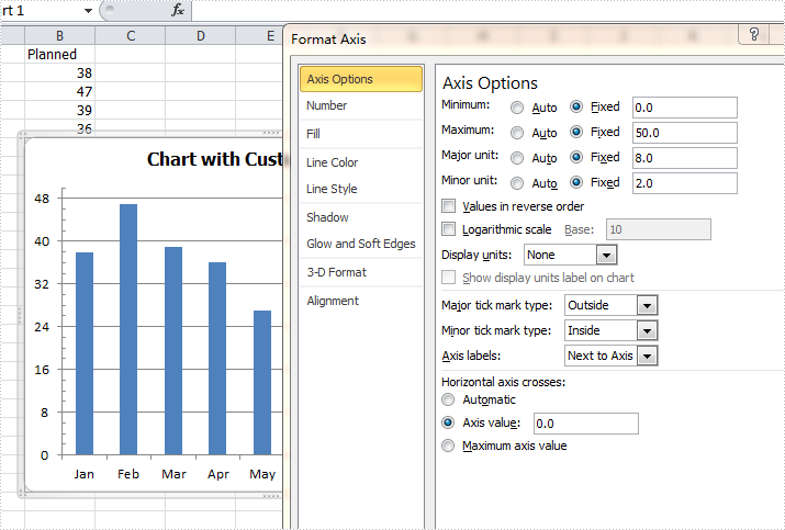
By default, Excel sets the axis properties automatically for charts. These properties include axis options like maximum & minimum value, major & minor unit, major & minor tick mark type, axis labels position, axis across value and whether values in reverse order. Sometimes we need to set those properties manually to beautify and perfect the charts. This article is going to introduce the method to customize axis setting for Excel chart in C# using Spire.XLS.
Note: before start, please download the latest version of Spire.XLS and add the .dll in the bin folder as the reference of Visual Studio.
Step 1: Create a workbook and add a sheet filled with some sample data.
            Workbook workbook = new Workbook();
            workbook.CreateEmptySheets(1);
            Worksheet sheet = workbook.Worksheets[0];
            sheet.Name = "Demo";
            sheet.Range["A1"].Value = "Month";
            sheet.Range["A2"].Value = "Jan";
            sheet.Range["A3"].Value = "Feb";
            sheet.Range["A4"].Value = "Mar";
            sheet.Range["A5"].Value = "Apr";
            sheet.Range["A6"].Value = "May";
            sheet.Range["A7"].Value = "Jun";
            sheet.Range["A8"].Value = "Jul";
            sheet.Range["A9"].Value = "Aug";
            sheet.Range["B1"].Value = "Planned";
            sheet.Range["B2"].NumberValue = 38;
            sheet.Range["B3"].NumberValue = 47;
            sheet.Range["B4"].NumberValue = 39;
            sheet.Range["B5"].NumberValue = 36;
            sheet.Range["B6"].NumberValue = 27;
            sheet.Range["B7"].NumberValue = 25;
            sheet.Range["B8"].NumberValue = 36;
            sheet.Range["B9"].NumberValue = 48;
Step 2: Create a column clustered chart based on the sample data.
            Chart chart = sheet.Charts.Add(ExcelChartType.ColumnClustered);
            chart.DataRange = sheet.Range["B1:B9"];
            chart.SeriesDataFromRange = false;
            chart.PlotArea.Visible = false;
            chart.TopRow = 6;
            chart.BottomRow = 25;
            chart.LeftColumn = 2;
            chart.RightColumn = 9;
            chart.ChartTitle = "Chart with Customized Axis";
            chart.ChartTitleArea.IsBold = true;
            chart.ChartTitleArea.Size = 12;
            Spire.Xls.Charts.ChartSerie cs1 = chart.Series[0];
            cs1.CategoryLabels = sheet.Range["A2:A9"];
Step 3: Set the customized axis properties for the chart.
            chart.PrimaryValueAxis.MajorUnit = 8;
            chart.PrimaryValueAxis.MinorUnit = 2;
            chart.PrimaryValueAxis.MaxValue = 50;
            chart.PrimaryValueAxis.MinValue = 0;
            chart.PrimaryValueAxis.IsReverseOrder = false;
            chart.PrimaryValueAxis.MajorTickMark = TickMarkType.TickMarkOutside;
            chart.PrimaryValueAxis.MinorTickMark = TickMarkType.TickMarkInside;
            chart.PrimaryValueAxis.TickLabelPosition = TickLabelPositionType.TickLabelPositionNextToAxis;
            chart.PrimaryValueAxis.CrossesAt = 0;
Step 4: Save the document and launch to see effects.
            workbook.SaveToFile("Result.xlsx", ExcelVersion.Version2010);
            System.Diagnostics.Process.Start("Result.xlsx");
Effects:
Full codes:
using System;
using System.Collections.Generic;
using System.Linq;
using System.Text;
using Spire.Xls;
using System.Drawing;

namespace ConsoleApplication2
{
    class Program
    {
        static void Main(string[] args)
        {
            Workbook workbook = new Workbook();
            workbook.CreateEmptySheets(1);
            Worksheet sheet = workbook.Worksheets[0];
            sheet.Name = "Demo";
            sheet.Range["A1"].Value = "Month";
            sheet.Range["A2"].Value = "Jan";
            sheet.Range["A3"].Value = "Feb";
            sheet.Range["A4"].Value = "Mar";
            sheet.Range["A5"].Value = "Apr";
            sheet.Range["A6"].Value = "May";
            sheet.Range["A7"].Value = "Jun";
            sheet.Range["A8"].Value = "Jul";
            sheet.Range["A9"].Value = "Aug";
            sheet.Range["B1"].Value = "Planned";
            sheet.Range["B2"].NumberValue = 38;
            sheet.Range["B3"].NumberValue = 47;
            sheet.Range["B4"].NumberValue = 39;
            sheet.Range["B5"].NumberValue = 36;
            sheet.Range["B6"].NumberValue = 27;
            sheet.Range["B7"].NumberValue = 25;
            sheet.Range["B8"].NumberValue = 36;
            sheet.Range["B9"].NumberValue = 48;

            Chart chart = sheet.Charts.Add(ExcelChartType.ColumnClustered);
            chart.DataRange = sheet.Range["B1:B9"];
            chart.SeriesDataFromRange = false;
            chart.PlotArea.Visible = false;
            chart.TopRow = 6;
            chart.BottomRow = 25;
            chart.LeftColumn = 2;
            chart.RightColumn = 9;
            chart.ChartTitle = "Chart with Customized Axis";
            chart.ChartTitleArea.IsBold = true;
            chart.ChartTitleArea.Size = 12;
            Spire.Xls.Charts.ChartSerie cs1 = chart.Series[0];
            cs1.CategoryLabels = sheet.Range["A2:A9"];

            chart.PrimaryValueAxis.MajorUnit = 8;
            chart.PrimaryValueAxis.MinorUnit = 2;
            chart.PrimaryValueAxis.MaxValue = 50;
            chart.PrimaryValueAxis.MinValue = 0;
            chart.PrimaryValueAxis.IsReverseOrder = false;
            chart.PrimaryValueAxis.MajorTickMark = TickMarkType.TickMarkOutside;
            chart.PrimaryValueAxis.MinorTickMark = TickMarkType.TickMarkInside;
            chart.PrimaryValueAxis.TickLabelPosition = TickLabelPositionType.TickLabelPositionNextToAxis;
            chart.PrimaryValueAxis.CrossesAt = 0;

            workbook.SaveToFile("Result.xlsx", ExcelVersion.Version2010);
            System.Diagnostics.Process.Start("Result.xlsx");
        }
    }
}
Embed 3D Interactive Graphics into PDF Document in C#/VB.NET
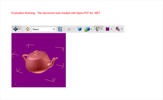
2015-09-22 08:43:39 Written by AdministratorUniversal 3D (U3D) is a compressed file format for 3D computer graphic data. 3D modules in U3D format can be inserted into PDF documents and interactively visualized by Acrobat Reader. This article presents how to embed a pre-created U3D file into a PDF document using Spire.PDF in C#, VB.NET.
Main Steps:
Step 1: Initialize a new object of PdfDocuemnt, and add a blank page to the PDF document.
PdfDocument doc = new PdfDocument();
PdfPageBase page = doc.Pages.Add();
Step 2: Draw a rectangle on the page to define the canvas area for the 3D file.
RectangleF rt = new RectangleF(0, 80, 200, 200);
Step 3: Initialize a new object of Pdf3DAnnotation, load the .u3d file as 3D annotation.
Pdf3DArtwork artwork = new Pdf3DArtwork("teapot.u3d", Pdf3DFileFormat.U3D);
Pdf3DAnnotation annotation = new Pdf3DAnnotation(page, rt, artwork);
annotation.Activation = new Pdf3DActivation();
annotation.Activation.ActivationMode = Pdf3DActivationMode.PageOpen;
Step 4: Define a 3D view mode.
Pdf3DView view = new Pdf3DView("test");
view.Background = new Pdf3DBackground(new PdfRGBColor(Color.Purple));
view.InternalName = "test";
view.RenderMode = new Pdf3DRenderMode(PdfRenderModeType.Solid);
view.LightingScheme = new Pdf3DLightingScheme(PdfLightingSchemeType.Day);
Step 5: Set the 3D view mode for the annotation.
annotation.Views.Add(view);
Step 6: Add the annotation to PDF.
PdfAnnotationCollection.Create(page).Add(annotation);
Step 7: Save the file.
doc.SaveToFile("Create3DPdf.pdf", FileFormat.PDF);
Output:
Full Code:
using Spire.Pdf;
using Spire.Pdf.Interactive.Annotations;
using Spire.Pdf.Multimedia._3DArtwork;
using Spire.Pdf.Graphics;
using System.Drawing;

namespace Embed3DInteractiveGraphics
{
    class Program
    {
        static void Main(string[] args)
        {
            PdfDocument doc = new PdfDocument();
            PdfPageBase page = doc.Pages.Add();

            RectangleF rt = new RectangleF(0, 80, 200, 200);
            Pdf3DArtwork artwork = new Pdf3DArtwork("teapot.u3d", Pdf3DFileFormat.U3D);
            Pdf3DAnnotation annotation = new Pdf3DAnnotation(page, rt, artwork);
            annotation.Activation = new Pdf3DActivation();
            annotation.Activation.ActivationMode = Pdf3DActivationMode.PageOpen;
            Pdf3DView view = new Pdf3DView("test");
            view.Background = new Pdf3DBackground(new PdfRGBColor(Color.Purple));
            view.InternalName = "test";
            view.RenderMode = new Pdf3DRenderMode(PdfRenderModeType.Solid);
            view.LightingScheme = new Pdf3DLightingScheme(PdfLightingSchemeType.Day);
            annotation.Views.Add(view);

            PdfAnnotationCollection.Create(page).Add(annotation);
            doc.SaveToFile("Create3DPdf.pdf", FileFormat.PDF);
        }
    }
}
Imports Spire.Pdf
Imports Spire.Pdf.Interactive.Annotations
Imports Spire.Pdf.Multimedia._3DArtwork
Imports Spire.Pdf.Graphics
Imports System.Drawing

Namespace Embed3DInteractiveGraphics
	Class Program
		Private Shared Sub Main(args As String())
			Dim doc As New PdfDocument()
			Dim page As PdfPageBase = doc.Pages.Add()

			Dim rt As New RectangleF(0, 80, 200, 200)
			Dim artwork As New Pdf3DArtwork("teapot.u3d", Pdf3DFileFormat.U3D)
			Dim annotation As New Pdf3DAnnotation(page, rt, artwork)
			annotation.Activation = New Pdf3DActivation()
			annotation.Activation.ActivationMode = Pdf3DActivationMode.PageOpen
			Dim view As New Pdf3DView("test")
			view.Background = New Pdf3DBackground(New PdfRGBColor(Color.Purple))
			view.InternalName = "test"
			view.RenderMode = New Pdf3DRenderMode(PdfRenderModeType.Solid)
			view.LightingScheme = New Pdf3DLightingScheme(PdfLightingSchemeType.Day)
			annotation.Views.Add(view)

			PdfAnnotationCollection.Create(page).Add(annotation)
			doc.SaveToFile("Create3DPdf.pdf", FileFormat.PDF)
		End Sub
	End Class
End Namespace
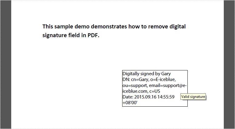
As a comprehensive PDF component, Spire.PDF supports to sign a PDF digitally, embed certificate in PDF as well as delete signatures in existing PDF documents. In this article, you'll learn how to remove all digital signatures from a PDF with C#, VB.NET.
Test File:
Code Snippet:
Step 1: Create a new PdfDocument object and load the test file.
PdfDocument pdf = new PdfDocument("test.pdf");
Step 2: Get loaded form from PDF.
PdfFormWidget widgets = pdf.Form as PdfFormWidget;
Step 3: Get the list of filed collection, and judge if each filed is a signature filed. If yes, remove the signature field using PdfFieldCollection.RemoveAt(int index) method.
for (int i = 0; i < widgets.FieldsWidget.List.Count; i++)
{
    PdfFieldWidget widget = widgets.FieldsWidget.List[i] as PdfFieldWidget;
    if (widget is PdfSignatureFieldWidget)
    {
        widgets.FieldsWidget.RemoveAt(i);
    }
}
Step 4: Save and launch the result file.
pdf.SaveToFile("result.pdf");
System.Diagnostics.Process.Start("result.pdf");
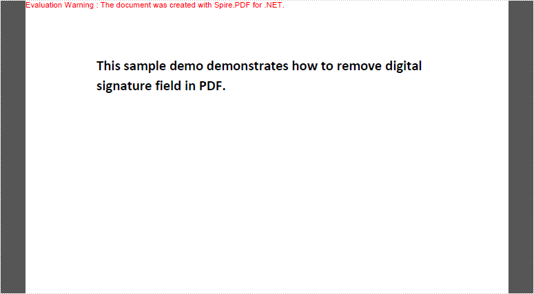
Result:
Full Code:
using Spire.Pdf;
using Spire.Pdf.Widget;

namespace RemoveDigitalSignature
{
    class Program
    {
        static void Main(string[] args)
        {
            PdfDocument pdf = new PdfDocument("test.pdf");

            PdfFormWidget widgets = pdf.Form as PdfFormWidget;
            for (int i = 0; i < widgets.FieldsWidget.List.Count; i++)
            {
                PdfFieldWidget widget = widgets.FieldsWidget.List[i] as PdfFieldWidget;
                if (widget is PdfSignatureFieldWidget)
                {
                    widgets.FieldsWidget.RemoveAt(i);
                }
            }

            pdf.SaveToFile("result.pdf");
            System.Diagnostics.Process.Start("result.pdf");
        }
    }
}
Imports Spire.Pdf
Imports Spire.Pdf.Widget

Namespace RemoveDigitalSignature
	Class Program
		Private Shared Sub Main(args As String())
			Dim pdf As New PdfDocument("test.pdf")
Dim widgets As PdfFormWidget = TryCast(pdf.Form, PdfFormWidget)
For i As Integer = 0 To widgets.FieldsWidget.List.Count - 1
	Dim widget As PdfFieldWidget = TryCast(widgets.FieldsWidget.List(i), PdfFieldWidget)
	If TypeOf widget Is PdfSignatureFieldWidget Then

		widgets.FieldsWidget.RemoveAt(i)
	End If
Next

pdf.SaveToFile("result.pdf")
System.Diagnostics.Process.Start("result.pdf")
		End Sub
	End Class
End Namespace
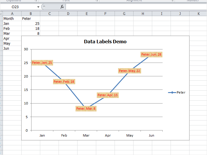
There are articles in our tutorials that introduce how to add trendline, error bars and data tables to Excel charts in C# using Spire.XLS. It's worthy of mention that Spire.XLS also supports data labels which are widely used to quickly identify a data series in a chart. In label options, we could set whether label contains series name, category name, value, percentages (pie chart) and legend key. This article is going to introduce the method to set and format data labels for Excel charts in C# using Spire.XLS.
Note: before start, please download the latest version of Spire.XLS and add the .dll in the bin folder as the reference of Visual Studio.
Step 1: Create an Excel document and add sample data.
            Workbook workbook = new Workbook();
            workbook.CreateEmptySheets(1);
            Worksheet sheet = workbook.Worksheets[0];
            sheet.Name = "Demo";
            sheet.Range["A1"].Value = "Month";
            sheet.Range["A2"].Value = "Jan";
            sheet.Range["A3"].Value = "Feb";
            sheet.Range["A4"].Value = "Mar";
            sheet.Range["A5"].Value = "Apr";
            sheet.Range["A6"].Value = "May";
            sheet.Range["A7"].Value = "Jun";
            sheet.Range["B1"].Value = "Peter";
            sheet.Range["B2"].NumberValue = 25;
            sheet.Range["B3"].NumberValue = 18;
            sheet.Range["B4"].NumberValue = 8;
            sheet.Range["B5"].NumberValue = 13;
            sheet.Range["B6"].NumberValue = 22;
            sheet.Range["B7"].NumberValue = 28;
Step 2: Create a line markers chart based on the sample data.
            Chart chart = sheet.Charts.Add(ExcelChartType.LineMarkers);
            chart.DataRange = sheet.Range["B1:B7"];
            chart.PlotArea.Visible = false;
            chart.SeriesDataFromRange = false;
            chart.TopRow = 5;
            chart.BottomRow = 26;
            chart.LeftColumn = 2;
            chart.RightColumn =11;
            chart.ChartTitle = "Data Labels Demo";
            chart.ChartTitleArea.IsBold = true;
            chart.ChartTitleArea.Size = 12;
            Spire.Xls.Charts.ChartSerie cs1 = chart.Series[0];
            cs1.CategoryLabels = sheet.Range["A2:A7"];
Step 3: Set which parts are displayed in the data labels and the delimiter to separate them.
            cs1.DataPoints.DefaultDataPoint.DataLabels.HasValue = true;
            cs1.DataPoints.DefaultDataPoint.DataLabels.HasLegendKey = false;
            cs1.DataPoints.DefaultDataPoint.DataLabels.HasPercentage = false;
            cs1.DataPoints.DefaultDataPoint.DataLabels.HasSeriesName = true;
            cs1.DataPoints.DefaultDataPoint.DataLabels.HasCategoryName = true;
            cs1.DataPoints.DefaultDataPoint.DataLabels.Delimiter = ". ";
Step 4: Set the font, position and fill effects for data labels in the chart.
            cs1.DataPoints.DefaultDataPoint.DataLabels.Size = 9;
            cs1.DataPoints.DefaultDataPoint.DataLabels.Color = Color.Red;
            cs1.DataPoints.DefaultDataPoint.DataLabels.FontName = "Calibri";
            cs1.DataPoints.DefaultDataPoint.DataLabels.Position = DataLabelPositionType.Center;
            cs1.DataPoints.DefaultDataPoint.DataLabels.FrameFormat.Fill.Texture = GradientTextureType.Papyrus;
Step 5: Save the document as Excel 2010.
            workbook.SaveToFile("S3.xlsx", ExcelVersion.Version2010);
            System.Diagnostics.Process.Start("S3.xlsx");
Effects:
Full Codes:
using System;
using System.Collections.Generic;
using System.Linq;
using System.Text;
using Spire.Xls;
using System.Drawing;

namespace ConsoleApplication2
{
    class Program
    {
        static void Main(string[] args)
        {

            Workbook workbook = new Workbook();
            workbook.CreateEmptySheets(1);
            Worksheet sheet = workbook.Worksheets[0];

            sheet.Name = "Demo";
            sheet.Range["A1"].Value = "Month";
            sheet.Range["A2"].Value = "Jan";
            sheet.Range["A3"].Value = "Feb";
            sheet.Range["A4"].Value = "Mar";
            sheet.Range["A5"].Value = "Apr";
            sheet.Range["A6"].Value = "May";
            sheet.Range["A7"].Value = "Jun";
            sheet.Range["B1"].Value = "Peter";
            sheet.Range["B2"].NumberValue = 25;
            sheet.Range["B3"].NumberValue = 18;
            sheet.Range["B4"].NumberValue = 8;
            sheet.Range["B5"].NumberValue = 13;
            sheet.Range["B6"].NumberValue = 22;
            sheet.Range["B7"].NumberValue = 28;

            Chart chart = sheet.Charts.Add(ExcelChartType.LineMarkers);
            chart.DataRange = sheet.Range["B1:B7"];
            chart.PlotArea.Visible = false;
            chart.SeriesDataFromRange = false;
            chart.TopRow = 5;
            chart.BottomRow = 26;
            chart.LeftColumn = 2;
            chart.RightColumn =11;
            chart.ChartTitle = "Data Labels Demo";
            chart.ChartTitleArea.IsBold = true;
            chart.ChartTitleArea.Size = 12;
            Spire.Xls.Charts.ChartSerie cs1 = chart.Series[0];
            cs1.CategoryLabels = sheet.Range["A2:A7"];

            cs1.DataPoints.DefaultDataPoint.DataLabels.HasValue = true;
            cs1.DataPoints.DefaultDataPoint.DataLabels.HasLegendKey = false;
            cs1.DataPoints.DefaultDataPoint.DataLabels.HasPercentage = false;
            cs1.DataPoints.DefaultDataPoint.DataLabels.HasSeriesName = true;
            cs1.DataPoints.DefaultDataPoint.DataLabels.HasCategoryName = true;
            cs1.DataPoints.DefaultDataPoint.DataLabels.Delimiter = ". ";

            cs1.DataPoints.DefaultDataPoint.DataLabels.Size = 9;
            cs1.DataPoints.DefaultDataPoint.DataLabels.Color = Color.Red;
            cs1.DataPoints.DefaultDataPoint.DataLabels.FontName = "Calibri";
            cs1.DataPoints.DefaultDataPoint.DataLabels.Position = DataLabelPositionType.Center;
            cs1.DataPoints.DefaultDataPoint.DataLabels.FrameFormat.Fill.Texture = GradientTextureType.Papyrus;

            workbook.SaveToFile("S3.xlsx", ExcelVersion.Version2010);
            System.Diagnostics.Process.Start("S3.xlsx");
        }
    }
}
As a powerful Excel library, Spire.XLS supports to work with many kinds of charts and it also supports to set the performance for the chart. We have already shown you how to fill the excel chart with background image to make the chart more attractive. This article will show you how to fill the excel chart with background color in C#.
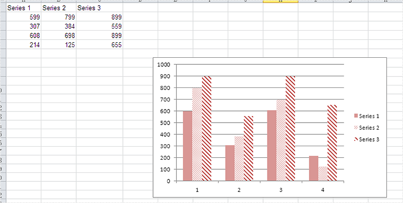
Please check the original Excel chart without any background color:
Code Snippet for Inserting Background color:
Step 1: Create a new workbook and load from file.
Workbook workbook = new Workbook();
workbook.LoadFromFile("sample.xlsx");
Step 2: Get the first worksheet from workbook and then get the first chart from the worksheet.
Worksheet ws = workbook.Worksheets[0];
Chart chart = ws.Charts[0];
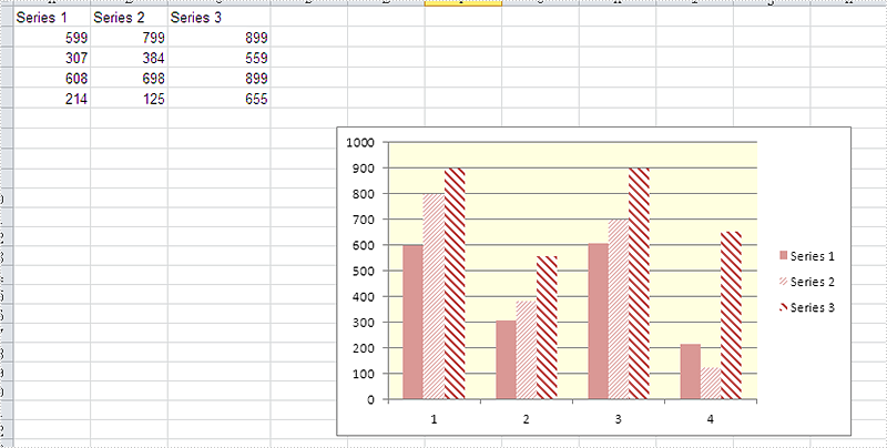
Step 3: Set the property to ForeGroundColor for PlotArea to fill the background color for the chart.
chart.PlotArea.ForeGroundColor = System.Drawing.Color.LightYellow;
Step 4: Save the document to file.
workbook.SaveToFile("result.xlsx",ExcelVersion.Version2010);
Effective screenshot after fill the background color for Excel chart:
Full codes:
using Spire.Xls;
namespace SetBackgroundColor
{
    class Program
    {

        static void Main(string[] args)
        {
            Workbook workbook = new Workbook();
            workbook.LoadFromFile("sample.xlsx");

            Worksheet ws = workbook.Worksheets[0];
            Chart chart = ws.Charts[0];

            chart.PlotArea.ForeGroundColor = System.Drawing.Color.LightYellow;

            workbook.SaveToFile("result.xlsx", ExcelVersion.Version2010);
        }

    }
}
Nowadays, we're facing a bigger chance to download a file from URL since more documents are electronically delivered by internet. In this article, I'll introduce how to download a Word document from URL programmatically using Spire.Doc in C#, VB.NET.
Spire.Doc does not provide a method to download a Word file directly from URL. However, you can download the file from URL into a MemoryStream and then use Spire.Doc to load the document from MemoryStream and save as a new Word document to local folder.
Code Snippet:
Step 1: Initialize a new Word document.
Document doc = new Document();
Step 2: Initialize a new instance of WebClient class.
WebClient webClient = new WebClient();
Step 3: Call WebClient.DownloadData(string address) method to load the data from URL. Save the data to a MemoryStream, then call Document.LoadFromStream() method to load the Word document from MemoryStream.
using (MemoryStream ms = new MemoryStream(webClient.DownloadData("http://www.e-iceblue.com/images/test.docx")))
{
    doc.LoadFromStream(ms,FileFormat.Docx);
}
Step 4: Save the file.
doc.SaveToFile("result.docx",FileFormat.Docx);
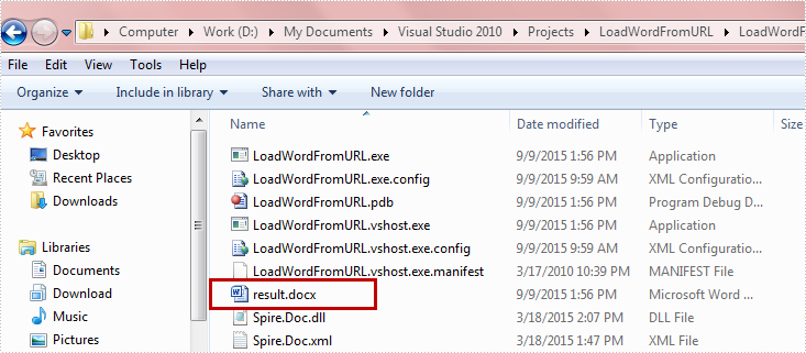
Run the program, the targeted file will be downloaded and saved as a new Word file in Bin folder.
Full Code:
using Spire.Doc;
using System.IO;
using System.Net;

namespace DownloadfromURL
{
    class Program
    {
        static void Main(string[] args)
        {
            Document doc = new Document();
            WebClient webClient = new WebClient();
            using (MemoryStream ms = new MemoryStream(webClient.DownloadData("http://www.e-iceblue.com/images/test.docx")))
            {
                doc.LoadFromStream(ms, FileFormat.Docx);
            }
            doc.SaveToFile("result.docx", FileFormat.Docx);
        }
    }
}
Imports Spire.Doc
Imports System.IO
Imports System.Net
Namespace DownloadfromURL
	Class Program
		Private Shared Sub Main(args As String())
			Dim doc As New Document()
			Dim webClient As New WebClient()
Using ms As New MemoryStream(webClient.DownloadData("http://www.e-iceblue.com/images/test.docx"))
				doc.LoadFromStream(ms, FileFormat.Docx)
			End Using
			doc.SaveToFile("result.docx", FileFormat.Docx)

		End Sub
	End Class
End Namespace
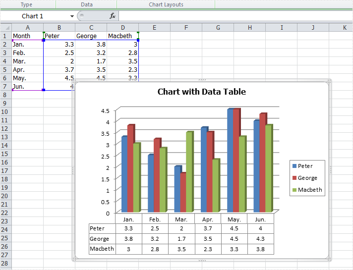
In Excel, we could use charts to visualize and compare data. However, once the charts are created, it becomes much difficult for us to read the data precisely from charts. Adding a data table below the chart is a good solution for which the chart and data are on the same place. This article is going to introduce the method to add a data table to the chart that is based on the data in C# using Spire.XLS.
Note: before start, please download the latest version of Spire.XLS and add the .dll in the bin folder as the reference of Visual studio.
Step 1: Create a new workbook and add an empty sheet.
            Workbook workbook = new Workbook();
            workbook.CreateEmptySheets(1);
            Worksheet sheet = workbook.Worksheets[0];
Step 2: Fill cells with sample data.
            sheet.Name = "Demo";
            sheet.Range["A1"].Value = "Month";
            sheet.Range["A2"].Value = "Jan.";
            sheet.Range["A3"].Value = "Feb.";
            sheet.Range["A4"].Value = "Mar.";
            sheet.Range["A5"].Value = "Apr.";
            sheet.Range["A6"].Value = "May.";
            sheet.Range["A7"].Value = "Jun.";
            sheet.Range["B1"].Value = "Peter";
            sheet.Range["B2"].NumberValue = 3.3;
            sheet.Range["B3"].NumberValue = 2.5;
            sheet.Range["B4"].NumberValue = 2.0;
            sheet.Range["B5"].NumberValue = 3.7;
            sheet.Range["B6"].NumberValue = 4.5;
            sheet.Range["B7"].NumberValue = 4.0;
            sheet.Range["C1"].Value = "George";
            sheet.Range["C2"].NumberValue = 3.8;
            sheet.Range["C3"].NumberValue = 3.2;
            sheet.Range["C4"].NumberValue = 1.7;
            sheet.Range["C5"].NumberValue = 3.5;
            sheet.Range["C6"].NumberValue = 4.5;
            sheet.Range["C7"].NumberValue = 4.3;
            sheet.Range["D1"].Value = "Macbeth";
            sheet.Range["D2"].NumberValue = 3.0;
            sheet.Range["D3"].NumberValue = 2.8;
            sheet.Range["D4"].NumberValue = 3.5;
            sheet.Range["D5"].NumberValue = 2.3;
            sheet.Range["D6"].NumberValue = 3.3;
            sheet.Range["D7"].NumberValue = 3.8;
Step 3: Create a Column3DClustered based on the sample data.
            Chart chart = sheet.Charts.Add(ExcelChartType.Column3DClustered);
            chart.DataRange = sheet.Range["B1:D7"];
            chart.SeriesDataFromRange = false;
            chart.TopRow = 7;
            chart.BottomRow = 28;
            chart.LeftColumn = 3;
            chart.RightColumn =11;
            chart.ChartTitle = "Chart with Data Table";
            chart.ChartTitleArea.IsBold = true;
            chart.ChartTitleArea.Size = 12;
            Spire.Xls.Charts.ChartSerie cs1 = chart.Series[0];
            cs1.CategoryLabels = sheet.Range["A2:A7"];
Step 4: Add a data table to the chart that is based on the data.
chart.HasDataTable = true;
Step 5: Save the document and launch to see effects.
            workbook.SaveToFile("S3.xlsx", ExcelVersion.Version2010);
            System.Diagnostics.Process.Start("S3.xlsx");
Effects:
Full codes:
using System;
using System.Collections.Generic;
using System.Linq;
using System.Text;
using Spire.Xls;
using System.Drawing;

namespace ConsoleApplication2
{
    class Program
    {
        static void Main(string[] args)
        {

            Workbook workbook = new Workbook();
            workbook.CreateEmptySheets(1);
            Worksheet sheet = workbook.Worksheets[0];

            sheet.Name = "Demo";
            sheet.Range["A1"].Value = "Month";
            sheet.Range["A2"].Value = "Jan.";
            sheet.Range["A3"].Value = "Feb.";
            sheet.Range["A4"].Value = "Mar.";
            sheet.Range["A5"].Value = "Apr.";
            sheet.Range["A6"].Value = "May.";
            sheet.Range["A7"].Value = "Jun.";
            sheet.Range["B1"].Value = "Peter";
            sheet.Range["B2"].NumberValue = 3.3;
            sheet.Range["B3"].NumberValue = 2.5;
            sheet.Range["B4"].NumberValue = 2.0;
            sheet.Range["B5"].NumberValue = 3.7;
            sheet.Range["B6"].NumberValue = 4.5;
            sheet.Range["B7"].NumberValue = 4.0;
            sheet.Range["C1"].Value = "George";
            sheet.Range["C2"].NumberValue = 3.8;
            sheet.Range["C3"].NumberValue = 3.2;
            sheet.Range["C4"].NumberValue = 1.7;
            sheet.Range["C5"].NumberValue = 3.5;
            sheet.Range["C6"].NumberValue = 4.5;
            sheet.Range["C7"].NumberValue = 4.3;
            sheet.Range["D1"].Value = "Macbeth";
            sheet.Range["D2"].NumberValue = 3.0;
            sheet.Range["D3"].NumberValue = 2.8;
            sheet.Range["D4"].NumberValue = 3.5;
            sheet.Range["D5"].NumberValue = 2.3;
            sheet.Range["D6"].NumberValue = 3.3;
            sheet.Range["D7"].NumberValue = 3.8;

            Chart chart = sheet.Charts.Add(ExcelChartType.Column3DClustered);
            chart.DataRange = sheet.Range["B1:D7"];
            chart.SeriesDataFromRange = false;
            chart.TopRow = 7;
            chart.BottomRow = 28;
            chart.LeftColumn = 3;
            chart.RightColumn =11;
            chart.ChartTitle = "Chart with Data Table";
            chart.ChartTitleArea.IsBold = true;
            chart.ChartTitleArea.Size = 12;
            Spire.Xls.Charts.ChartSerie cs1 = chart.Series[0];
            cs1.CategoryLabels = sheet.Range["A2:A7"];
            chart.HasDataTable = true;

            workbook.SaveToFile("S3.xlsx", ExcelVersion.Version2010);
            System.Diagnostics.Process.Start("S3.xlsx");
        }
    }
}
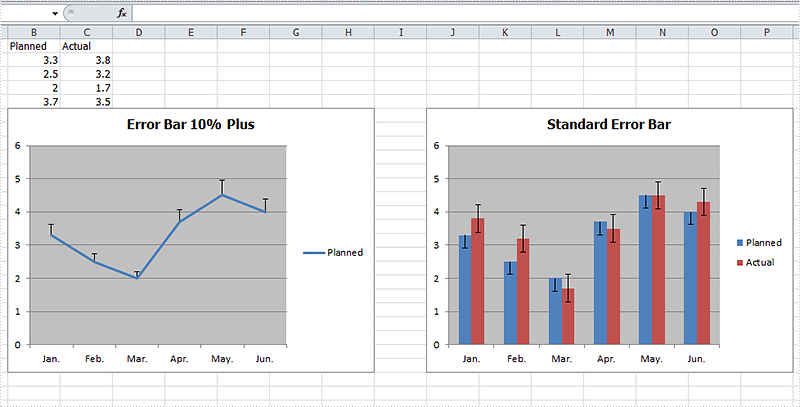
Error bars are a graphical representation of the variability of data and helps us see margins of error and standard deviations immediately in charts with a standard error amount, a percentage, a standard deviation or a custom error amount. Error bars can be used in 2-D area, bar, column, line, scatter, and bubble charts, which are all supported by Spire.XLS. This article is going to introduce the method to add error bars to a chart in C# using Spire.XLS.
Note: before start, please download the latest version of Spire.XLS and add the .dll in the bin folder as the reference of Visual Studio.
Step 1: Create a workbook and fill the sample data in sheet.
            Workbook workbook = new Workbook();
            workbook.CreateEmptySheets(1);
            Worksheet sheet = workbook.Worksheets[0];
            sheet.Name = "Demo";
            sheet.Range["A1"].Value = "Month";
            sheet.Range["A2"].Value = "Jan.";
            sheet.Range["A3"].Value = "Feb.";
            sheet.Range["A4"].Value = "Mar.";
            sheet.Range["A5"].Value = "Apr.";
            sheet.Range["A6"].Value = "May.";
            sheet.Range["A7"].Value = "Jun.";
            sheet.Range["B1"].Value = "Planned";
            sheet.Range["B2"].NumberValue = 3.3;
            sheet.Range["B3"].NumberValue = 2.5;
            sheet.Range["B4"].NumberValue = 2.0;
            sheet.Range["B5"].NumberValue = 3.7;
            sheet.Range["B6"].NumberValue = 4.5;
            sheet.Range["B7"].NumberValue = 4.0;
            sheet.Range["C1"].Value = "Actual";
            sheet.Range["C2"].NumberValue = 3.8;
            sheet.Range["C3"].NumberValue = 3.2;
            sheet.Range["C4"].NumberValue = 1.7;
            sheet.Range["C5"].NumberValue = 3.5;
            sheet.Range["C6"].NumberValue = 4.5;
            sheet.Range["C7"].NumberValue = 4.3;
Step 2: Add a line chart and then add percentage error bar to the chart. The direction of error bars can be set as both, minus and plus and the type of error bars can be set as fixed value, percentage, standard deviation, standard error or custom. After setting the direction and type, we can set the amount.
            Chart chart = sheet.Charts.Add(ExcelChartType.Line);
            chart.DataRange = sheet.Range["B1:B7"];
            chart.SeriesDataFromRange = false;
            chart.TopRow = 6;
            chart.BottomRow = 25;
            chart.LeftColumn = 2;
            chart.RightColumn = 9;
            chart.ChartTitle = "Error Bar 10% Plus";
            chart.ChartTitleArea.IsBold = true;
            chart.ChartTitleArea.Size = 12;
            Spire.Xls.Charts.ChartSerie cs1 = chart.Series[0];
            cs1.CategoryLabels = sheet.Range["A2:A7"];
            cs1.ErrorBar(true, ErrorBarIncludeType.Plus, ErrorBarType.Percentage,10);
Step 3: Add a column chart with standard error bars as comparison.
            Chart chart2 = sheet.Charts.Add(ExcelChartType.ColumnClustered);
            chart2.DataRange = sheet.Range["B1:C7"];
            chart2.SeriesDataFromRange = false;
            chart2.TopRow = 6;
            chart2.BottomRow = 25;
            chart2.LeftColumn = 10;
            chart2.RightColumn = 17;
            chart2.ChartTitle = "Standard Error Bar";
            chart2.ChartTitleArea.IsBold = true;
            chart2.ChartTitleArea.Size = 12;
            Spire.Xls.Charts.ChartSerie cs2 = chart2.Series[0];
            cs2.CategoryLabels = sheet.Range["A2:A7"];
            cs2.ErrorBar(true, ErrorBarIncludeType.Minus, ErrorBarType.StandardError, 0.3);
            Spire.Xls.Charts.ChartSerie cs3 = chart2.Series[1];
            cs3.ErrorBar(true, ErrorBarIncludeType.Both, ErrorBarType.StandardError, 0.5);
Step 4: Save the document and launch to see effects.
            workbook.SaveToFile("S3.xlsx", ExcelVersion.Version2010);
            System.Diagnostics.Process.Start("S3.xlsx");
Effects:
Full Codes:
using System;
using System.Collections.Generic;
using System.Linq;
using System.Text;
using Spire.Xls;
using System.Drawing;

namespace ConsoleApplication2
{
    class Program
    {
        static void Main(string[] args)
        {

            Workbook workbook = new Workbook();
            workbook.CreateEmptySheets(1);
            Worksheet sheet = workbook.Worksheets[0];
            sheet.Name = "Demo";
            sheet.Range["A1"].Value = "Month";
            sheet.Range["A2"].Value = "Jan.";
            sheet.Range["A3"].Value = "Feb.";
            sheet.Range["A4"].Value = "Mar.";
            sheet.Range["A5"].Value = "Apr.";
            sheet.Range["A6"].Value = "May.";
            sheet.Range["A7"].Value = "Jun.";
            sheet.Range["B1"].Value = "Planned";
            sheet.Range["B2"].NumberValue = 3.3;
            sheet.Range["B3"].NumberValue = 2.5;
            sheet.Range["B4"].NumberValue = 2.0;
            sheet.Range["B5"].NumberValue = 3.7;
            sheet.Range["B6"].NumberValue = 4.5;
            sheet.Range["B7"].NumberValue = 4.0;
            sheet.Range["C1"].Value = "Actual";
            sheet.Range["C2"].NumberValue = 3.8;
            sheet.Range["C3"].NumberValue = 3.2;
            sheet.Range["C4"].NumberValue = 1.7;
            sheet.Range["C5"].NumberValue = 3.5;
            sheet.Range["C6"].NumberValue = 4.5;
            sheet.Range["C7"].NumberValue = 4.3;

            Chart chart = sheet.Charts.Add(ExcelChartType.Line);
            chart.DataRange = sheet.Range["B1:B7"];
            chart.SeriesDataFromRange = false;
            chart.TopRow = 6;
            chart.BottomRow = 25;
            chart.LeftColumn = 2;
            chart.RightColumn = 9;
            chart.ChartTitle = "Error Bar 10% Plus";
            chart.ChartTitleArea.IsBold = true;
            chart.ChartTitleArea.Size = 12;
            Spire.Xls.Charts.ChartSerie cs1 = chart.Series[0];
            cs1.CategoryLabels = sheet.Range["A2:A7"];
            cs1.ErrorBar(true, ErrorBarIncludeType.Plus, ErrorBarType.Percentage,10);

            Chart chart2 = sheet.Charts.Add(ExcelChartType.ColumnClustered);
            chart2.DataRange = sheet.Range["B1:C7"];
            chart2.SeriesDataFromRange = false;
            chart2.TopRow = 6;
            chart2.BottomRow = 25;
            chart2.LeftColumn = 10;
            chart2.RightColumn = 17;
            chart2.ChartTitle = "Standard Error Bar";
            chart2.ChartTitleArea.IsBold = true;
            chart2.ChartTitleArea.Size = 12;
            Spire.Xls.Charts.ChartSerie cs2 = chart2.Series[0];
            cs2.CategoryLabels = sheet.Range["A2:A7"];
            cs2.ErrorBar(true, ErrorBarIncludeType.Minus, ErrorBarType.StandardError, 0.3);
            Spire.Xls.Charts.ChartSerie cs3 = chart2.Series[1];
            cs3.ErrorBar(true, ErrorBarIncludeType.Both, ErrorBarType.StandardError, 0.5);

            workbook.SaveToFile("S3.xlsx", ExcelVersion.Version2010);
            System.Diagnostics.Process.Start("S3.xlsx");

        }
    }
}
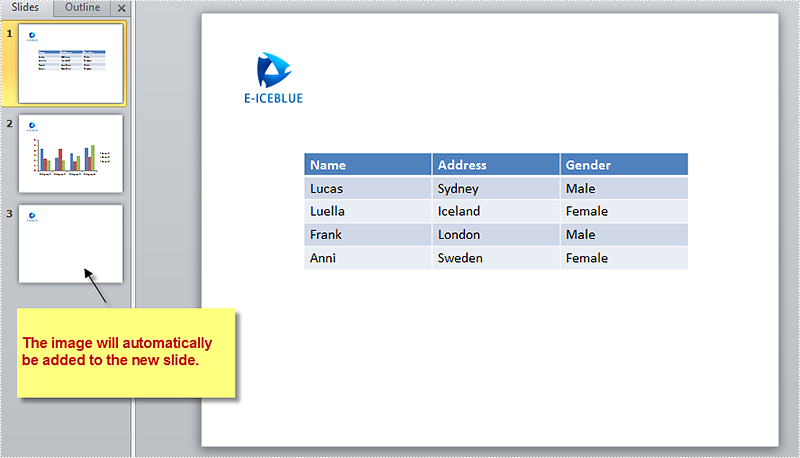
A slide master is the top slide that stores the information about the theme and slide layouts, which will be inherited by other slides in the presentation. In other words, when you modify the style of slide master, every slide in the presentation will be changed accordingly, including the ones added later.
This quality makes it possible that when you want to insert an image or watermark to every slide, you only need to insert the image in slide master. In this article, you'll learn how to add an image to slide master using Spire.Presenation in C#, VB.NET.
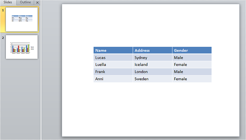
Screenshot of original file:
Detailed Steps:
Step 1: Initialize a new Presentation and load the sample file
Presentation presentation = new Presentation();
presentation.LoadFromFile(@"sample.pptx");
Step 2: Get the master collection.
IMasterSlide master = presentation.Masters[0];
Step 3: Insert an image to slide master.
String image = @"logo.png";
RectangleF rff = new RectangleF(40, 40, 100, 80);
IEmbedImage pic=master.Shapes.AppendEmbedImage(ShapeType.Rectangle, image, rff);
pic.Line.FillFormat.FillType = FillFormatType.None;
Step 4: Add a new blank slide to the presentation.
presentation.Slides.Append();
Step 5: Save and launch the file.
presentation.SaveToFile("result.pptx", FileFormat.Pptx2010);
System.Diagnostics.Process.Start("result.pptx");
Output:
Full Code:
using Spire.Presentation;
using Spire.Presentation.Drawing;
using System;
using System.Drawing;

namespace AddImage
{

    class Program
    {

        static void Main(string[] args)
        {
            //initialize a new Presentation and load the sample file
            Presentation presentation = new Presentation();
            presentation.LoadFromFile(@"sample.pptx");
            //get the master collection
            IMasterSlide master = presentation.Masters[0];
            //append image to slide master
            String image = @"logo.png";
            RectangleF rff = new RectangleF(40, 40, 100, 80);
            IEmbedImage pic = master.Shapes.AppendEmbedImage(ShapeType.Rectangle, image, rff);
            pic.Line.FillFormat.FillType = FillFormatType.None;
            //add new slide to presentation
            presentation.Slides.Append();
            //save and launch the file
            presentation.SaveToFile("result.pptx", FileFormat.Pptx2010);
            System.Diagnostics.Process.Start("result.pptx");
        }
    }
}
Imports Spire.Presentation
Imports Spire.Presentation.Drawing
Imports System.Drawing

Namespace AddImage

	Class Program

		Private Shared Sub Main(args As String())
			'initialize a new Presentation and load the sample file
			Dim presentation As New Presentation()
			presentation.LoadFromFile("sample.pptx")
			'get the master collection
			Dim master As IMasterSlide = presentation.Masters(0)
			'append image to slide master
			Dim image As [String] = "logo.png"
			Dim rff As New RectangleF(40, 40, 100, 80)
			Dim pic As IEmbedImage = master.Shapes.AppendEmbedImage(ShapeType.Rectangle, image, rff)
			pic.Line.FillFormat.FillType = FillFormatType.None
			'add new slide to presentation
			presentation.Slides.Append()
			'save and launch the file
			presentation.SaveToFile("result.pptx", FileFormat.Pptx2010)
			System.Diagnostics.Process.Start("result.pptx")
		End Sub
	End Class
End Namespace
How to format cells with borders in conditional formatting
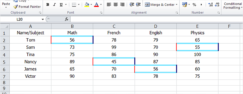
2015-08-31 01:31:47 Written by AdministratorUsing conditional formatting in Excel, we could highlight interesting cells, emphasize unusual values and visualize data with Data Bars, Color Scales and Icon Sets based on criteria. In the two articles Alternate Row Colors in Excel with Conditional Formatting and Apply Conditional Formatting to a Data Range, we have introduce the method to set fill, font, data bars, color scales and icon sets in conditional formatting using Spire.XLS. This article is going to introduce the method to format cells with borders in conditional formatting.
Note: before start, please download the latest version of Spire.XLS and add the .dll in the bin folder as the reference of Visual Studio.
Step 1: Create a new workbook and add sample data.
            Workbook workbook = new Workbook();
            Worksheet sheet = workbook.Worksheets[0];

            sheet.Range["A1"].Value = "Name/Subject";
            sheet.Range["A2"].Value = "Tom";
            sheet.Range["A3"].Value = "Sam";
            sheet.Range["A4"].Value = "Tina";
            sheet.Range["A5"].Value = "Nancy";
            sheet.Range["A6"].Value = "James";
            sheet.Range["A7"].Value = "Victor";
            sheet.Range["B1"].Value = "Math";
            sheet.Range["C1"].Value = "French";
            sheet.Range["D1"].Value = "English";
            sheet.Range["E1"].Value = "Physics";
            sheet.Range["B2"].NumberValue = 56;
            sheet.Range["B3"].NumberValue = 73;
            sheet.Range["B4"].NumberValue = 75;
            sheet.Range["B5"].NumberValue = 89;
            sheet.Range["B6"].NumberValue = 65;
            sheet.Range["B7"].NumberValue = 90;
            sheet.Range["C2"].NumberValue = 78;
            sheet.Range["C3"].NumberValue = 99;
            sheet.Range["C4"].NumberValue = 86;
            sheet.Range["C5"].NumberValue = 45;
            sheet.Range["C6"].NumberValue = 70;
            sheet.Range["C7"].NumberValue = 83;
            sheet.Range["D2"].NumberValue = 79;
            sheet.Range["D3"].NumberValue = 70;
            sheet.Range["D4"].NumberValue = 90;
            sheet.Range["D5"].NumberValue = 87;
            sheet.Range["D6"].NumberValue = 56;
            sheet.Range["D7"].NumberValue = 78;
            sheet.Range["E2"].NumberValue = 65;
            sheet.Range["E3"].NumberValue = 55;
            sheet.Range["E4"].NumberValue = 100;
            sheet.Range["E5"].NumberValue = 85;
            sheet.Range["E6"].NumberValue = 60;
            sheet.Range["E7"].NumberValue = 75;

            sheet.AllocatedRange.RowHeight = 17;
            sheet.AllocatedRange.ColumnWidth = 17;
            sheet.AllocatedRange.VerticalAlignment = VerticalAlignType.Center;
            sheet.AllocatedRange.HorizontalAlignment = HorizontalAlignType.Center;
Step 2: Set the formatting rule using formula. Here the rule is the number values less than 60.
XlsConditionalFormats xcfs1 = sheet.ConditionalFormats.Add();
xcfs1.AddRange(sheet.Range["B2:E7"]);
IConditionalFormat format1 = xcfs1.AddCondition();
format1.FormatType = ConditionalFormatType.CellValue;
format1.FirstFormula = "60";
format1.Operator = ComparisonOperatorType.Less;
Step 3: Set border colors and styles for cells that match the condition.
            format1.LeftBorderColor = Color.Red;
            format1.RightBorderColor = Color.DarkBlue;
            format1.TopBorderColor = Color.DeepSkyBlue;
            format1.BottomBorderColor = Color.DeepSkyBlue;

            format1.LeftBorderStyle = LineStyleType.Medium;
            format1.RightBorderStyle = LineStyleType.Thick;
            format1.TopBorderStyle = LineStyleType.Double;
            format1.BottomBorderStyle = LineStyleType.Double;
Step 4: Save the document and launch to see effects.
            workbook.SaveToFile("sample.xlsx", ExcelVersion.Version2010);
            System.Diagnostics.Process.Start("sample.xlsx");
Effects:
Full Codes:
using Spire.Xls;
using Spire.Xls.Core;
using Spire.Xls.Core.Spreadsheet.Collections;
using System.Drawing;

namespace ApplyConditionalFormatting
{
    class Program
    {
        static void Main(string[] args)
        {
            Workbook workbook = new Workbook();
            Worksheet sheet = workbook.Worksheets[0];

            sheet.Range["A1"].Value = "Name/Subject";
            sheet.Range["A2"].Value = "Tom";
            sheet.Range["A3"].Value = "Sam";
            sheet.Range["A4"].Value = "Tina";
            sheet.Range["A5"].Value = "Nancy";
            sheet.Range["A6"].Value = "James";
            sheet.Range["A7"].Value = "Victor";
            sheet.Range["B1"].Value = "Math";
            sheet.Range["C1"].Value = "French";
            sheet.Range["D1"].Value = "English";
            sheet.Range["E1"].Value = "Physics";
            sheet.Range["B2"].NumberValue = 56;
            sheet.Range["B3"].NumberValue = 73;
            sheet.Range["B4"].NumberValue = 75;
            sheet.Range["B5"].NumberValue = 89;
            sheet.Range["B6"].NumberValue = 65;
            sheet.Range["B7"].NumberValue = 90;
            sheet.Range["C2"].NumberValue = 78;
            sheet.Range["C3"].NumberValue = 99;
            sheet.Range["C4"].NumberValue = 86;
            sheet.Range["C5"].NumberValue = 45;
            sheet.Range["C6"].NumberValue = 70;
            sheet.Range["C7"].NumberValue = 83;
            sheet.Range["D2"].NumberValue = 79;
            sheet.Range["D3"].NumberValue = 70;
            sheet.Range["D4"].NumberValue = 90;
            sheet.Range["D5"].NumberValue = 87;
            sheet.Range["D6"].NumberValue = 56;
            sheet.Range["D7"].NumberValue = 78;
            sheet.Range["E2"].NumberValue = 65;
            sheet.Range["E3"].NumberValue = 55;
            sheet.Range["E4"].NumberValue = 100;
            sheet.Range["E5"].NumberValue = 85;
            sheet.Range["E6"].NumberValue = 60;
            sheet.Range["E7"].NumberValue = 75;

            sheet.AllocatedRange.RowHeight = 17;
            sheet.AllocatedRange.ColumnWidth = 17;
            sheet.AllocatedRange.VerticalAlignment = VerticalAlignType.Center;
            sheet.AllocatedRange.HorizontalAlignment = HorizontalAlignType.Center;

            // Apply conditional formatting to the score range (B2:E7)
            XlsConditionalFormats xcfs1 = sheet.ConditionalFormats.Add();
            xcfs1.AddRange(sheet.Range["B2:E7"]);

            // Highlight cells with scores less than 60 using custom borders
            IConditionalFormat format1 = xcfs1.AddCondition();
            format1.FormatType = ConditionalFormatType.CellValue; // Compare cell values
            format1.FirstFormula = "60";
            format1.Operator = ComparisonOperatorType.Less;

            // Set border colors
            format1.LeftBorderColor = Color.Red;
            format1.RightBorderColor = Color.DarkBlue;
            format1.TopBorderColor = Color.DeepSkyBlue;
            format1.BottomBorderColor = Color.DeepSkyBlue;

            // Set border styles
            format1.LeftBorderStyle = LineStyleType.Medium;
            format1.RightBorderStyle = LineStyleType.Thick;
            format1.TopBorderStyle = LineStyleType.Double;
            format1.BottomBorderStyle = LineStyleType.Double;

            workbook.SaveToFile("sample.xlsx", ExcelVersion.Version2010);
            System.Diagnostics.Process.Start("sample.xlsx");
        }
    }
}
