C#/VB.NET: Create a Waterfall Chart in Excel
Waterfall charts in Excel are graphs that visually show how a series of consecutive positive or negative values contribute to the final outcome. They are a useful tool for tracking company profits or cash flow, comparing product revenues, analyzing sales and inventory changes over time, etc. In this article, you will learn how to create a waterfall chart in Excel in C# and VB.NET using Spire.XLS for .NET.
Install Spire.XLS for .NET
To begin with, you need to add the DLL files included in the Spire.XLS for .NET package as references in your .NET project. The DLL files can be either downloaded from this link or installed via NuGet.
PM> Install-Package Spire.XLS
Create a Waterfall Chart in Excel in C# and VB.NET
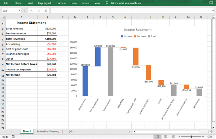
Waterfall/bridge charts are ideal for analyzing financial statements. To add a waterfall chart to an Excel worksheet, Spire.XLS for .NET provides the Worksheet.Charts.Add(ExcelChartType.WaterFall) method. The following are the detailed steps.
- Create a Workbook instance.
- Load a sample Excel document using Workbook.LoadFromFile() method.
- Get a specified worksheet by its index using Workbook.Worksheets[sheetIndex] property.
- Add a waterfall chart to the worksheet using Worksheet.Charts.Add(ExcelChartType.WaterFall) method.
- Set data range for the chart using Chart.DataRange property.
- Set position and title of the chart.
- Get a specified data series of the chart and then set specific data points in the chart as totals or subtotals using ChartSerie.DataPoints[int index].SetAsTotal property.
- Show the connector lines between data points by setting the ChartSerie.Format.ShowConnectorLines property to true.
- Show data labels for data points, and set the legend position of the chart.
- Save the result document using Workbook.SaveToFile() method.
- C#
- VB.NET
using Spire.Xls;

namespace WaterfallChart
{
    class Program
    {
        static void Main(string[] args)
        {
            //Create a Workbook instance
            Workbook workbook = new Workbook();

            //Load a sample Excel document
            workbook.LoadFromFile("Data.xlsx");

            //Get the first worksheet
            Worksheet sheet = workbook.Worksheets[0];

            //Add a waterfall chart to the the worksheet
            Chart chart = sheet.Charts.Add(ExcelChartType.WaterFall);

            //Set data range for the chart
            chart.DataRange = sheet["A2:B11"];

            //Set position of the chart
            chart.LeftColumn = 4;
            chart.TopRow = 2;
            chart.RightColumn = 15;
            chart.BottomRow = 23;

            //Set the chart title
            chart.ChartTitle = "Income Statement";

            //Set specific data points in the chart as totals or subtotals
            chart.Series[0].DataPoints[2].SetAsTotal = true;
            chart.Series[0].DataPoints[7].SetAsTotal = true;
            chart.Series[0].DataPoints[9].SetAsTotal = true;

            //Show the connector lines between data points
            chart.Series[0].Format.ShowConnectorLines = true;

            //Show data labels for data points
            chart.Series[0].DataPoints.DefaultDataPoint.DataLabels.HasValue = true;
            chart.Series[0].DataPoints.DefaultDataPoint.DataLabels.Size = 8;

            //Set the legend position of the chart
            chart.Legend.Position = LegendPositionType.Top;

            //Save the result document
            workbook.SaveToFile("WaterfallChart.xlsx");
        }
    }
}
Apply for a Temporary License
If you'd like to remove the evaluation message from the generated documents, or to get rid of the function limitations, please request a 30-day trial license for yourself.
Create Bubble Chart in Excel in C#/VB.NET
This article will show you how to use Spire.XLS for .NET to create a bubble chart in Excel in C# and VB.NET.
using Spire.Xls;

namespace BubbleChart
{
    class Program
    {
        static void Main(string[] args)

        {
            //Create a new workbook
            Workbook workbook = new Workbook();

            //Add a worksheet and set name
            workbook.CreateEmptySheets(1);
            Worksheet sheet = workbook.Worksheets[0];
            sheet.Name = "Chart data";
            //Initialize chart and set its type
            Chart chart = sheet.Charts.Add(ExcelChartType.Bubble);

            //Set the position of the chart in the worksheet
            chart.LeftColumn = 1;
            chart.RightColumn = 10;
            chart.TopRow = 1;
            chart.BottomRow = 20;

            //Set title for the chart and values
            Spire.Xls.Charts.ChartSerie cs1 = chart.Series.Add("Bubble Chart");
            cs1.EnteredDirectlyValues = new object[] { 2.2, 5.6 };
            cs1.EnteredDirectlyCategoryLabels = new object[] { 1.1, 4.4 };
            cs1.EnteredDirectlyBubbles = new object[] { 3, 6 };

            //Save the document to file
            workbook.SaveToFile("Output.xlsx", ExcelVersion.Version2010);
        }
    }

}
Imports Spire.Xls

Namespace BubbleChart

    Class Program

        Private Shared Sub Main(ByVal args() As String)
            'Create a new workbook
            Dim workbook As Workbook = New Workbook
            'Add a worksheet and set name
            workbook.CreateEmptySheets(1)
            Dim sheet As Worksheet = workbook.Worksheets(0)
            sheet.Name = "Chart data"
            'Initialize chart and set its type
            Dim chart As Chart = sheet.Charts.Add(ExcelChartType.Bubble)
            'Set the position of the chart in the worksheet
            chart.LeftColumn = 1
            chart.RightColumn = 10
            chart.TopRow = 1
            chart.BottomRow = 20
            'Set title for the chart and values
            Dim cs1 As Spire.Xls.Charts.ChartSerie = chart.Series.Add("Bubble Chart")
            cs1.EnteredDirectlyValues = New Object() {2.2, 5.6}
            cs1.EnteredDirectlyCategoryLabels = New Object() {1.1, 4.4}
            cs1.EnteredDirectlyBubbles = New Object() {3, 6}
            'Save the document to file
            workbook.SaveToFile("Output.xlsx", ExcelVersion.Version2010)
        End Sub
    End Class
End Namespace
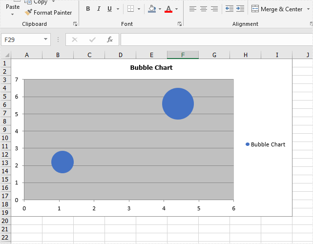
Effective screenshot of Excel Bubble chart:
Create Pivot Chart in Excel in C#
Starting from version 9.8.5, Spire.XLS supports creating pivot chart based on pivot table. This article is going to demonstrate how we can use Spire.XLS to implement this feature.
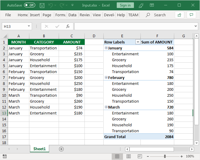
The input.xlsx Excel file:
Sample Code
using Spire.Xls;
using Spire.Xls.Core;

namespace CreatePivotChart
{
    class Program
    {
        static void Main(string[] args)
        {
            //load the Excel file
            Workbook workbook = new Workbook();
            workbook.LoadFromFile("Input.xlsx");

            //get the first worksheet
            Worksheet sheet = workbook.Worksheets[0];
            //get the first pivot table in the worksheet
            IPivotTable pivotTable = sheet.PivotTables[0];

            //create a clustered column chart based on the pivot table
            Chart chart = sheet.Charts.Add(ExcelChartType.ColumnClustered, pivotTable);
            //set chart position
            chart.TopRow = 19;
            chart.BottomRow = 38;
            //set chart title
            chart.ChartTitle = "Pivot Chart";

            //save the resultant file
            workbook.SaveToFile("CreatPivotChart.xlsx", ExcelVersion.Version2013);
        }
    }
}
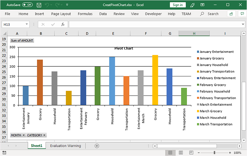
Screenshot of the created pivot chart:
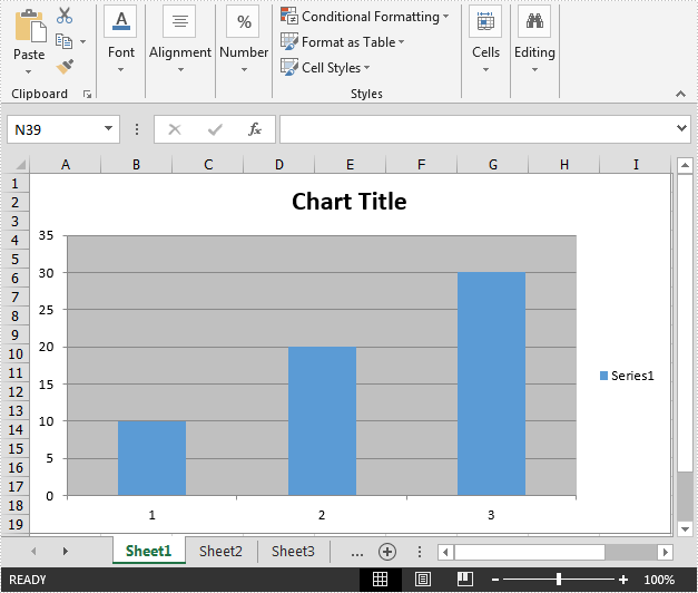
Create Chart without Using Worksheet Data Range in C#
This article demonstrates how to create a chart without reference to the worksheet data range using Spire.XLS.
Detail steps:
Step 1: Create a workbook and get the first worksheet.
Workbook wb = new Workbook();
Worksheet sheet = wb.Worksheets[0];
Step 2: Add a chart to the worksheet.
Chart chart = sheet.Charts.Add();
Step 3: Add a series to the chart.
var series = chart.Series.Add();
Step 4: Add data.
series.EnteredDirectlyValues = new object[] { 10, 20, 30 };
Step 5: Save the file.
wb.SaveToFile("result.xlsx", ExcelVersion.Version2013);
Output:
Full code:
using Spire.Xls;

namespace Create_chart
{
    class Program
    {
        static void Main(string[] args)
        {
            //Create a workbook
            Workbook wb = new Workbook();

            //Get the first worksheet
            Worksheet sheet = wb.Worksheets[0];

            //Add a chart to the worksheet
            Chart chart = sheet.Charts.Add();

            //Add a series to the chart
            var series = chart.Series.Add();

            //Add data
            series.EnteredDirectlyValues = new object[] { 10, 20, 30 };

            //Save the file
            wb.SaveToFile("result.xlsx", ExcelVersion.Version2013);
        }
    }
}
Apply Soft Edges effect to Excel Chart in C#
This article elaborates the steps to apply soft edges effect to an excel chart using Spire.XLS.
The example Excel file we used for demonstration:
Detail steps:
Step 1: Instantiate a Workbook object and load the excel file.
Workbook workbook = new Workbook();
workbook.LoadFromFile("Input.xlsx");
Step 2: Get the first worksheet.
Worksheet sheet = workbook.Worksheets[0];
Step 3: Get the chart.
IChart chart = sheet.Charts[0];
Step 4: Specify the size of the soft edge. Value can be set from 0 to 100.
chart.ChartArea.Shadow.SoftEdge = 10;
Step 5: Save the file.
workbook.SaveToFile("Output.xlsx", ExcelVersion.Version2013);
Output:
Full code:
using Spire.Xls;
using Spire.Xls.Core;

namespace Soft_Edges_in_Excel_Chart
{
    class Program
    {
        static void Main(string[] args)
        {
            //Instantiate a Workbook object
            Workbook workbook = new Workbook();
            //Load the Excel file
            workbook.LoadFromFile("Input.xlsx");

            //Get the first worksheet
            Worksheet sheet = workbook.Worksheets[0];

            //Get the chart
            IChart chart = sheet.Charts[0];

            //Specify the size of the soft edge. Value can be set from 0 to 100
            chart.ChartArea.Shadow.SoftEdge = 10;

            //Save the file
            workbook.SaveToFile("Output.xlsx", ExcelVersion.Version2013);
        }
    }
}
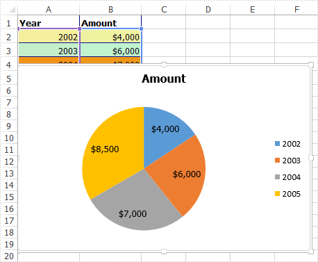
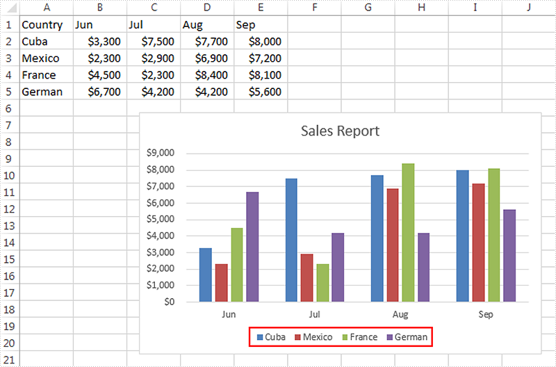
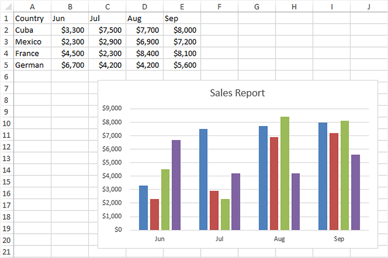
Delete Legend and Specific Legend Entries from Excel Chart in C#
A legend is displayed in the chart area by default. However it can be removed from the chart. With Spire.XLS, we can delete the whole legend as well as specific legend entries from Excel chart. This article is going to demonstrate how we can use Spire.XLS to accomplish this function.
Below screenshot shows the Excel chart we used for demonstration:
Delete the whole legend
using Spire.Xls;
namespace DeleteLegend
{

    class Program
    {

        static void Main(string[] args)
        {
            //Create a Workbook instance
            Workbook workbook = new Workbook();
            //Load the Excel file
            workbook.LoadFromFile("sample.xlsx");

            //Get the first worksheet
            Worksheet sheet = workbook.Worksheets[0];

            //Get the chart
            Chart chart = sheet.Charts[0];

            //Delete legend from the chart
            chart.Legend.Delete();

            //Save the file
            workbook.SaveToFile("DeleteLegend.xlsx", ExcelVersion.Version2013);
        }
    }
}
Screenshot:
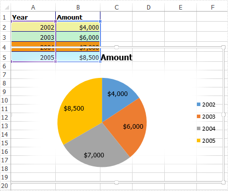
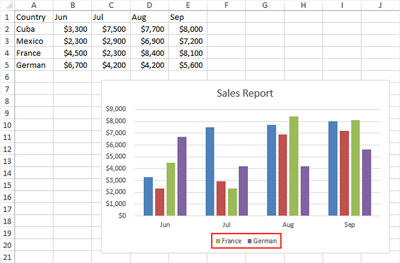
Delete specific legend entries
using Spire.Xls;
namespace DeleteLegend
{

    class Program
    {

        static void Main(string[] args)
        {
            //Create a Workbook instance
            Workbook workbook = new Workbook();
            //Load the Excel file
            workbook.LoadFromFile("sample.xlsx");

            //Get the first worksheet
            Worksheet sheet = workbook.Worksheets[0];

            //Get the chart
            Chart chart = sheet.Charts[0];

            //Delete the first and the second legend entries from the chart
            chart.Legend.LegendEntries[0].Delete();
            chart.Legend.LegendEntries[1].Delete();

            //Save the file
            workbook.SaveToFile("DeleteLegendEntries.xlsx", ExcelVersion.Version2013);

        }
    }
}
Screenshot:
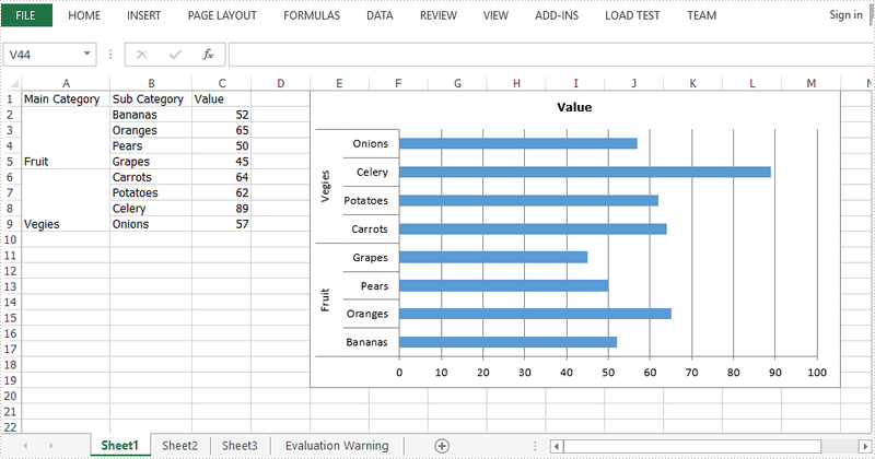
Create Multi-Level Category Chart in Excel in C#, VB.NET
Multi-level category chart is a chart type that has both main category and subcategory labels. This type of chart is useful when you have figures for items that belong to different categories. In this article, you will learn how to create a multi-level category chart in Excel using Spire.XLS with C# and VB.NET.
Step 1: Create a Workbook instance and get the first worksheet.
Workbook wb = new Workbook();
Worksheet sheet = wb.Worksheets[0];
Step 2: Write data to cells.
sheet.Range["A1"].Text = "Main Category";
sheet.Range["A2"].Text = "Fruit";
sheet.Range["A6"].Text = "Vegies";
sheet.Range["B1"].Text = "Sub Category";
sheet.Range["B2"].Text = "Bananas";
sheet.Range["B3"].Text = "Oranges";
sheet.Range["B4"].Text = "Pears";
sheet.Range["B5"].Text = "Grapes";
sheet.Range["B6"].Text = "Carrots";
sheet.Range["B7"].Text = "Potatoes";
sheet.Range["B8"].Text = "Celery";
sheet.Range["B9"].Text = "Onions";
sheet.Range["C1"].Text = "Value";
sheet.Range["C2"].Value = "52";
sheet.Range["C3"].Value = "65";
sheet.Range["C4"].Value = "50";
sheet.Range["C5"].Value = "45";
sheet.Range["C6"].Value = "64";
sheet.Range["C7"].Value = "62";
sheet.Range["C8"].Value = "89";
sheet.Range["C9"].Value = "57";
Step 3: Vertically merge cells from A2 to A5, A6 to A9.
sheet.Range["A2:A5"].Merge();
sheet.Range["A6:A9"].Merge();
Step 4: Add a clustered bar chart to worksheet.
Chart chart = sheet.Charts.Add(ExcelChartType.BarClustered);
chart.ChartTitle = "Value";
chart.PlotArea.Fill.FillType = ShapeFillType.NoFill;
chart.Legend.Delete();
Step 5: Set the data source of series data.
chart.DataRange = sheet.Range["C2:C9"];
chart.SeriesDataFromRange = false;
Step 6: Set the data source of category labels.
ChartSerie serie = chart.Series[0];
serie.CategoryLabels = sheet.Range["A2:B9"];
Step 7: Show multi-level category labels.
chart.PrimaryCategoryAxis.MultiLevelLable = true;
Step 8: Save the file.
wb.SaveToFile("output.xlsx", ExcelVersion.Version2013);
Output:
Full Code:
using Spire.Xls;
using Spire.Xls.Charts;
namespace CreateMutilLevelChart
{

    class Program
    {

        static void Main(string[] args)
        {
            Workbook wb = new Workbook();
            Worksheet sheet = wb.Worksheets[0];

            sheet.Range["A1"].Text = "Main Category";
            sheet.Range["A2"].Text = "Fruit";
            sheet.Range["A6"].Text = "Vegies";
            sheet.Range["B1"].Text = "Sub Category";
            sheet.Range["B2"].Text = "Bananas";
            sheet.Range["B3"].Text = "Oranges";
            sheet.Range["B4"].Text = "Pears";
            sheet.Range["B5"].Text = "Grapes";
            sheet.Range["B6"].Text = "Carrots";
            sheet.Range["B7"].Text = "Potatoes";
            sheet.Range["B8"].Text = "Celery";
            sheet.Range["B9"].Text = "Onions";
            sheet.Range["C1"].Text = "Value";
            sheet.Range["C2"].Value = "52";
            sheet.Range["C3"].Value = "65";
            sheet.Range["C4"].Value = "50";
            sheet.Range["C5"].Value = "45";
            sheet.Range["C6"].Value = "64";
            sheet.Range["C7"].Value = "62";
            sheet.Range["C8"].Value = "89";
            sheet.Range["C9"].Value = "57";
            sheet.Range["A2:A5"].Merge();
            sheet.Range["A6:A9"].Merge();
            sheet.AutoFitColumn(1);
            sheet.AutoFitColumn(2);

            Chart chart = sheet.Charts.Add(ExcelChartType.BarClustered);
            chart.ChartTitle = "Value";
            chart.PlotArea.Fill.FillType = ShapeFillType.NoFill;
            chart.Legend.Delete();
            chart.LeftColumn = 5;
            chart.TopRow = 1;
            chart.RightColumn = 14;
            chart.DataRange = sheet.Range["C2:C9"];
            chart.SeriesDataFromRange = false;
            ChartSerie serie = chart.Series[0];
            serie.CategoryLabels = sheet.Range["A2:B9"];
            chart.PrimaryCategoryAxis.MultiLevelLable = true;
            wb.SaveToFile("output.xlsx", ExcelVersion.Version2013);
        }
    }
}
Imports Spire.Xls
Imports Spire.Xls.Charts
Namespace CreateMutilLevelChart

	Class Program

		Private Shared Sub Main(args As String())
			Dim wb As New Workbook()
			Dim sheet As Worksheet = wb.Worksheets(0)

			sheet.Range("A1").Text = "Main Category"
			sheet.Range("A2").Text = "Fruit"
			sheet.Range("A6").Text = "Vegies"
			sheet.Range("B1").Text = "Sub Category"
			sheet.Range("B2").Text = "Bananas"
			sheet.Range("B3").Text = "Oranges"
			sheet.Range("B4").Text = "Pears"
			sheet.Range("B5").Text = "Grapes"
			sheet.Range("B6").Text = "Carrots"
			sheet.Range("B7").Text = "Potatoes"
			sheet.Range("B8").Text = "Celery"
			sheet.Range("B9").Text = "Onions"
			sheet.Range("C1").Text = "Value"
			sheet.Range("C2").Value = "52"
			sheet.Range("C3").Value = "65"
			sheet.Range("C4").Value = "50"
			sheet.Range("C5").Value = "45"
			sheet.Range("C6").Value = "64"
			sheet.Range("C7").Value = "62"
			sheet.Range("C8").Value = "89"
			sheet.Range("C9").Value = "57"
			sheet.Range("A2:A5").Merge()
			sheet.Range("A6:A9").Merge()
			sheet.AutoFitColumn(1)
			sheet.AutoFitColumn(2)

			Dim chart As Chart = sheet.Charts.Add(ExcelChartType.BarClustered)
			chart.ChartTitle = "Value"
			chart.PlotArea.Fill.FillType = ShapeFillType.NoFill
			chart.Legend.Delete()
			chart.LeftColumn = 5
			chart.TopRow = 1
			chart.RightColumn = 14
			chart.DataRange = sheet.Range("C2:C9")
			chart.SeriesDataFromRange = False
			Dim serie As ChartSerie = chart.Series(0)
			serie.CategoryLabels = sheet.Range("A2:B9")
			chart.PrimaryCategoryAxis.MultiLevelLable = True
			wb.SaveToFile("output.xlsx", ExcelVersion.Version2013)
		End Sub
	End Class
End Namespace
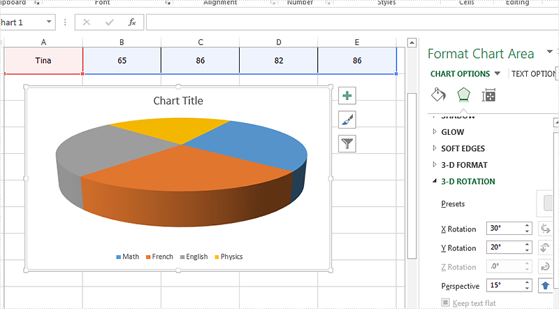
How to set the rotation for the 3D chart on Excel in C#
With Spire.XLS, we can set the 3-D rotation easily in C#. The following code example explains how to set the rotation of the 3D chart view in C#. We will use 3D pie chart for example. Firstly, view the original 3D pie chart:
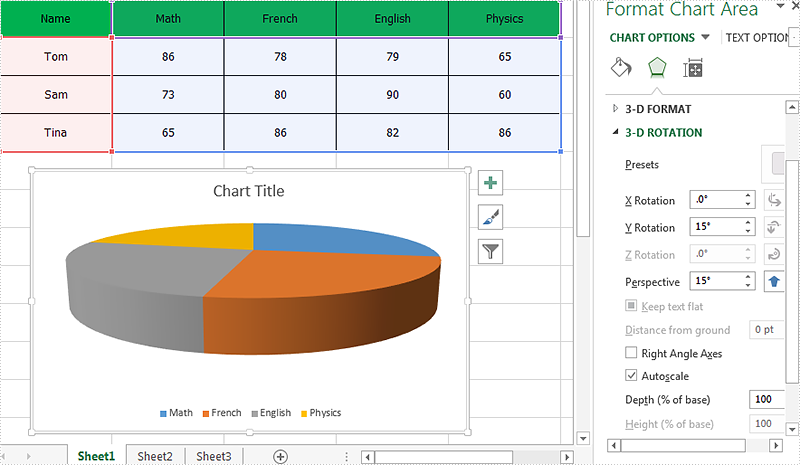
Code snippet of how to set the 3D rotation for Excel Chart:
Step 1: Create a new instance of workbook and load the sample document from file.
Workbook workbook = new Workbook();
workbook.LoadFromFile("Sample.xlsx");
Step 2: Get the chart from the first worksheet.
Worksheet sheet = workbook.Worksheets[0];
Chart chart = sheet.Charts[0];
Step 3: Set Rotation of the 3D chart view for X and Y.
//X rotation:
chart.Rotation=30;
//Y rotation:
chart.Elevation = 20;
Step 4: Save the document to file.
workbook.SaveToFile("Result.xlsx", ExcelVersion.Version2010);
Effective screenshot of the Excel 3D chart rotation:
Full codes:
using Spire.Xls;
namespace SetRotation
{

    class Program
    {

        static void Main(string[] args)
        {
            Workbook workbook = new Workbook();
            workbook.LoadFromFile("Sample.xlsx");

            Worksheet sheet = workbook.Worksheets[0];
            Chart chart = sheet.Charts[0];

            //X rotation:
            chart.Rotation = 30;
            //Y rotation:
            chart.Elevation = 20;

            workbook.SaveToFile("Result.xlsx", ExcelVersion.Version2010);
        }
    }
}
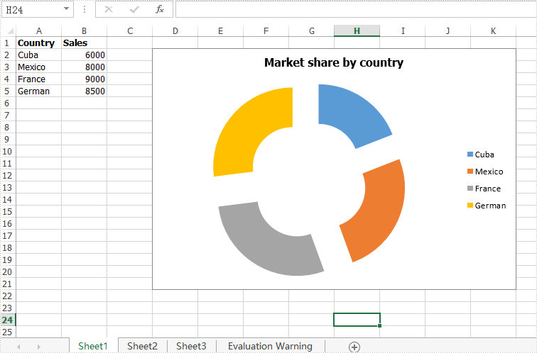
How to explode a doughnut chart in C#
In the previous article, we have demonstrated how to explode a pie chart via Spire.XLS. This article we will explain how to explode a doughnut chart in C#.
When we need to explode a doughnut chart, we can set the chart type as DoughnutExploded when we create a doughnut chart from scratch. For the existing doughnut chart, we can easily change the chart type to explode the doughnut chart.
Step 1: Create an instance of Excel workbook and load the document from file.
Workbook workbook = new Workbook();
workbook.LoadFromFile("DoughnutChart.xlsx",ExcelVersion.Version2010);
Step 2: Get the first worksheet from the sample workbook.
Worksheet sheet = workbook.Worksheets[0];
Step 3: Get the first chart from the first worksheet.
Chart chart = sheet.Charts[0];
Step 4: Set the chart type as DoughnutExploded to explode the doughnut chart.
chart.ChartType = ExcelChartType.DoughnutExploded;
Step 5: Save the document to file.
workbook.SaveToFile("ExplodedDoughnutChart.xlsx", ExcelVersion.Version2010);
Effective screenshot of the explode doughnut chart:
Full codes of how to explode a doughnut chart:
using Spire.Xls;
namespace ExplodeDoughnut
{

    class Program
    {

        static void Main(string[] args)
        {
            Workbook workbook = new Workbook();
            workbook.LoadFromFile("DoughnutChart.xlsx", ExcelVersion.Version2010);

            Worksheet sheet = workbook.Worksheets[0];
            Chart chart = sheet.Charts[0];
            chart.ChartType = ExcelChartType.DoughnutExploded;

            workbook.SaveToFile("ExplodedDoughnutChart.xlsx", ExcelVersion.Version2010);
        }

    }
}
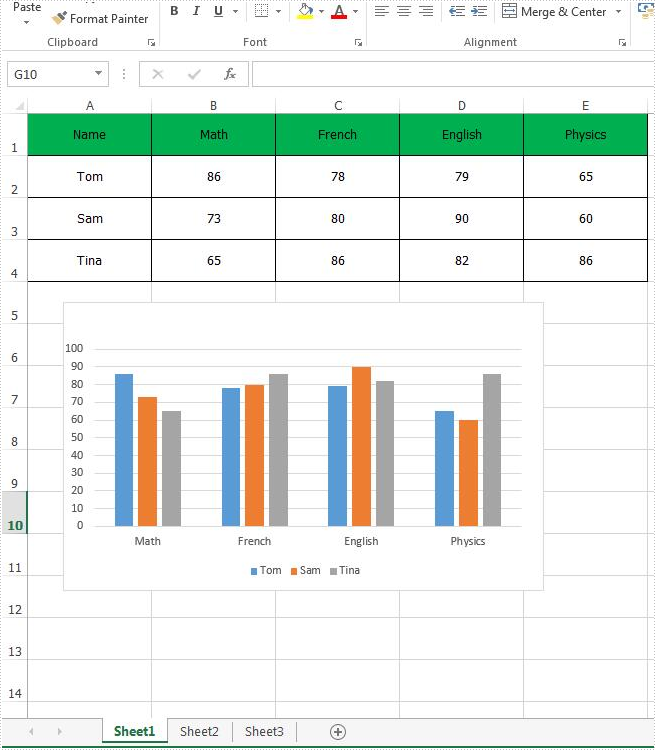
How to remove chart from Excel worksheet in C#, VB.NET
With Spire.XLS for .NET, we could easily add different kinds of charts to Excel worksheet, such as Pie Chart, Column Chart, bar chart, line chart, radar chart, Doughnut chart, pyramid chart, etc. In this article, we'll show you how to remove chart from Excel worksheet by using Spire.XLS.
Below is a sample document which contains a chart and table from the Excel worksheet, then we'll remove the chart from the slide.
C# Code Snippet of how to remove the chart from Excel:
Step 1: Create an instance of Excel workbook and load the document from file.
Workbook workbook = new Workbook();
workbook.LoadFromFile("Sample.xlsx");
Step 2: Get the first worksheet from the workbook.
Worksheet sheet = workbook.Worksheets[0];
Step 3: Get the first chart from the first worksheet.
IChartShape chart = sheet.Charts[0];
Step 4: Remove the chart.
chart.Remove();
Step 5: Save the document to file.
workbook.SaveToFile("RemoveChart.xlsx");
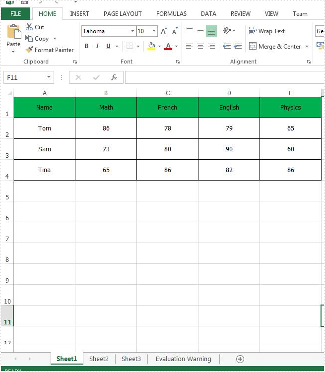
Effective screenshot:
Full code:
using Spire.Xls;
using Spire.Xls.Core;
namespace RemoveChart
{

    class Program
    {

        static void Main(string[] args)
        {
            Workbook workbook = new Workbook();
            workbook.LoadFromFile("Sample.xlsx");
            Worksheet sheet = workbook.Worksheets[0];
            IChartShape chart = sheet.Charts[0];
            chart.Remove();
            workbook.SaveToFile("RemoveChart.xlsx");

        }

    }
}
Imports Spire.Xls
Imports Spire.Xls.Core
Namespace RemoveChart

	Class Program

		Private Shared Sub Main(args As String())
			Dim workbook As New Workbook()
			workbook.LoadFromFile("Sample.xlsx")
			Dim sheet As Worksheet = workbook.Worksheets(0)
			Dim chart As IChartShape = sheet.Charts(0)
			chart.Remove()
			workbook.SaveToFile("RemoveChart.xlsx")

		End Sub

	End Class
End Namespace