
Conditional Formatting (11)
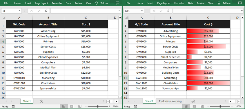
Data bars in Excel are a built-in type of conditional formatting that inserts colored bars in cells to compare the values within them. The length of a bar depends on the value of a cell and the longest bar corresponds to the largest value in a selected data range, which allows you to spot it at a glance. In this article, you will learn how to add data bars in a cell range using Spire.XLS for .NET.
Install Spire.XLS for .NET
To begin with, you need to add the DLL files included in the Spire.XLS for .NET package as references in your .NET project. The DLL files can be either downloaded from this link or installed via NuGet.
PM> Install-Package Spire.XLS
Add Data Bars in Excel in C# and VB.NET
Data bars are a great tool for visually comparing data within a selected range of cells. With Spire.XLS for .NET, you are allowed to add a data bar to a specified data range and also set its format. The following are the detailed steps.
- Create a Workbook instance.
- Load a sample Excel document using Workbook.LoadFromFile() method.
- Get a specified worksheet using Workbook.Worsheets[index] property.
- Add a conditional formatting to the worksheet using Worksheet.ConditionalFormats.Add() method and return an object of XlsConditionalFormats class.
- Set the cell range where the conditional formatting will be applied using XlsConditionalFormats.AddRange() method.
- Add a condition using XlsConditionalFormats.AddCondition() method, and then set its format type to DataBar using IConditionalFormat.FormatType property.
- Set the fill effect and color of the data bars using IConditionalFormat.DataBar.BarFillType and IConditionalFormat.DataBar.BarColor properties.
- Save the result document using Workbook.SaveToFile() method.
- C#
- VB.NET
using Spire.Xls;
using Spire.Xls.Core;
using Spire.Xls.Core.Spreadsheet.Collections;
using Spire.Xls.Core.Spreadsheet.ConditionalFormatting;
using System.Drawing;

namespace ApplyDataBar
{
    class Program
    {
        static void Main(string[] args)
        {
            //Create a Workbook instance
            Workbook workbook = new Workbook();

            //Load a sample Excel docuemnt
            workbook.LoadFromFile("sample.xlsx");

            //Get the first worksheet
            Worksheet sheet = workbook.Worksheets[0];

            //Add a conditional format to the worksheet
            XlsConditionalFormats xcfs = sheet.ConditionalFormats.Add();

            //Set the range where the conditional format will be applied
            xcfs.AddRange(sheet.Range["C2:C13"]);

            //Add a condition and set its format type to DataBar
            IConditionalFormat format = xcfs.AddCondition();
            format.FormatType = ConditionalFormatType.DataBar;

            //Set the fill effect and color of the data bars
            format.DataBar.BarFillType = DataBarFillType.DataBarFillGradient;
            format.DataBar.BarColor = Color.Red;

            //Save the result document
            workbook.SaveToFile("ApplyDataBarsToDataRange.xlsx", ExcelVersion.Version2013);
        }
    }
}
Apply for a Temporary License
If you'd like to remove the evaluation message from the generated documents, or to get rid of the function limitations, please request a 30-day trial license for yourself.
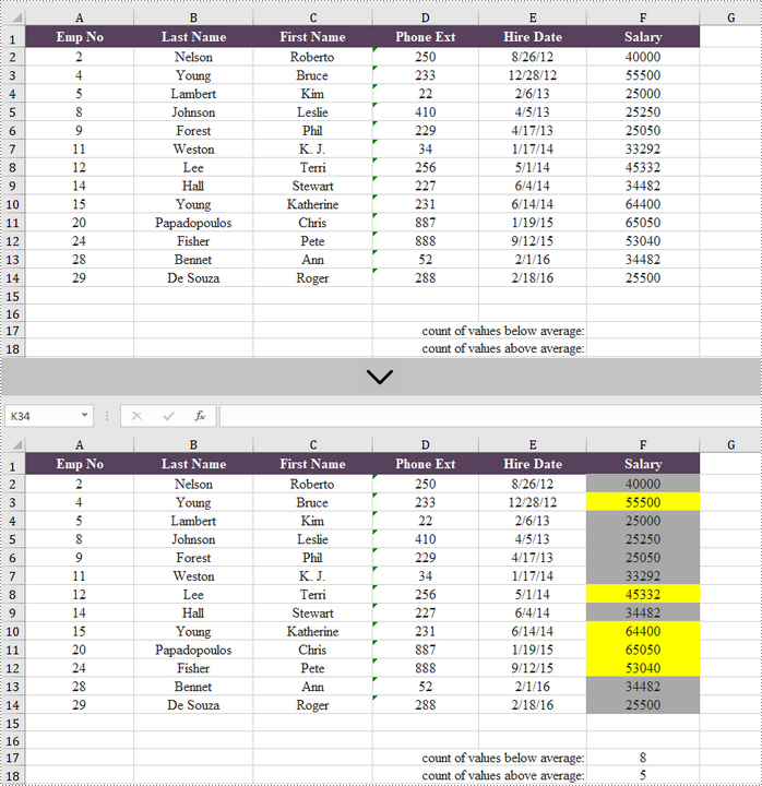
If you want to find values that are higher or lower than the average, you don't have to calculate the average, and then check those that are higher or lower. Using conditional formatting in Excel, you can automatically highlight those numbers. In this article, you will learn how to highlight values above average or below average with conditional formatting, by using Spire.XLS for .NET.
Install Spire.XLS for .NET
To begin with, you need to add the DLL files included in the Spire.XLS for .NET package as references in your .NET project. The DLL files can be either downloaded from this link or installed via NuGet.
PM> Install-Package Spire.XLS
Highlight Values Above or Below Average in Excel
Below are the steps to highlight values above or below average in Excel using Spire.XLS for .NET.
- Create a Workbook object.
- Load an Excel file using Workbook.LoadFromFile() method.
- Get a specific worksheet from the workbook through Workbook.Worsheets[index] property.
- Add a conditional formatting to the worksheet using Worksheet.ConditionalFormats.Add() method and return an object of XlsConditionalFormats class.
- Set the cell range where the conditional formatting will be applied using XlsConditionalFormats.AddRange() method.
- Add an average condition using XlsConditionalFormats.AddAverageCondition() method, specify the average type to above and change the background color of the cells that meet the condition to yellow.
- Add another average condition to change the background color of the below average values to dark gray.
- Save the workbook to an Excel file using Workbook.SaveToFile() method.
- C#
- VB.NET
using Spire.Xls;
using Spire.Xls.Core;
using Spire.Xls.Core.Spreadsheet.Collections;
using System.Drawing;

namespace HighlightValuesAboveAndBelowAverage
{
    class Program
    {
        static void Main(string[] args)
        {
            //Create a Workbook object
            Workbook workbook = new Workbook();

            //Load an Excel file
            workbook.LoadFromFile(@"C:\Users\Administrator\Desktop\sample.xlsx");

            //Get the first worksheet
            Worksheet sheet = workbook.Worksheets[0];

            //Add a conditional format to the worksheet
            XlsConditionalFormats format = sheet.ConditionalFormats.Add();

            //Set the range where the conditional format will be applied
            format.AddRange(sheet.Range["F2:F14"]);

            //Add a condition to highlight the top 2 ranked values
            IConditionalFormat condition1 = format.AddAverageCondition(AverageType.Above);
            condition1.BackColor = Color.Yellow;

            //Add a condition to highlight the bottom 2 ranked values
            IConditionalFormat condition2 = format.AddAverageCondition(AverageType.Below);
            condition2.BackColor = Color.DarkGray;

            //Get the count of values below average
            sheet.Range["F17"].Formula = "=COUNTIF(F2:F14,\"<\"&AVERAGE(F2:F14))";

            //Get the count of values above average
            sheet.Range["F18"].Formula = "=COUNTIF(F2:F14,\">\"&AVERAGE(F2:F14))";

            //Save the workbook to an Excel file
            workbook.SaveToFile("HighlightValues.xlsx", ExcelVersion.Version2016);
        }
    }
}
Apply for a Temporary License
If you'd like to remove the evaluation message from the generated documents, or to get rid of the function limitations, please request a 30-day trial license for yourself.
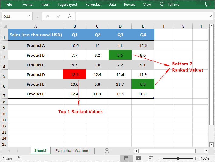
Searching for high or low values in large amounts of data can be cumbersome and error-prone. Fortunately, in Excel, you can apply conditional formatting to quickly highlight a specified number of top or bottom ranked values in a selected cell range. In this article, you will learn how to programmatically highlight top and bottom values in Excel using Spire.XLS for .NET.
Install Spire.XLS for .NET
To begin with, you need to add the DLL files included in the Spire.XLS for .NET package as references in your .NET project. The DLL files can be either downloaded from this link or installed via NuGet.
PM> Install-Package Spire.XLS
Highlight Top and Bottom Values in Excel in C# and VB.NET
Spire.XLS for .NET provides the XlsConditionalFormats.AddTopBottomCondition(TopBottomType topBottomType, int rank) method to specify the top N or bottom N ranked values, and then you can highlight these values with a background color. The following are the detailed steps.
- Create a Workbook instance.
- Load a sample Excel document using Workbook.LoadFromFile() method.
- Get a specified worksheet by its index using Workbook.Worksheets[sheetIndex] property.
- Add a conditional formatting to the worksheet using Worksheet.ConditionalFormats.Add() method and return an object of XlsConditionalFormats class.
- Set the cell range where the conditional formatting will be applied using XlsConditionalFormats.AddRange() method.
- Add a top condition to specify the highest or top N ranked values using XlsConditionalFormats.AddTopBottomCondition(TopBottomType topBottomType, int rank) method. Then highlight the cells that meet the condition with a background color using IConditionalFormat.BackColor property.
- Add a bottom condition to specify the lowest or bottom N ranked values and highlight the cells that meet the condition with a background color.
- Save the result document using Workbook.SaveToFile() method.
- C#
- VB.NET
using Spire.Xls;
using Spire.Xls.Core;
using Spire.Xls.Core.Spreadsheet.Collections;
using System.Drawing;

namespace HighlightValues
{
    class Program
    {
        static void Main(string[] args)
        {
            {

                //Create a Workbook instance
                Workbook workbook = new Workbook();

                //Load a sample Excel document
                workbook.LoadFromFile("sample.xlsx");

                //Get the first worksheet
                Worksheet sheet = workbook.Worksheets[0];

                //Add a conditional format to the worksheet
                XlsConditionalFormats format = sheet.ConditionalFormats.Add();

                //Set the range where the conditional format will be applied
                format.AddRange(sheet.Range["B2:F7"]);

                //Apply conditional formatting to highlight the highest values
                IConditionalFormat condition1 = format.AddTopBottomCondition(TopBottomType.Top, 1);
                condition1.BackColor = Color.Red;

                //Apply conditional formatting to highlight the bottom two values
                IConditionalFormat condition2 = format.AddTopBottomCondition(TopBottomType.Bottom, 2);
                condition2.BackColor = Color.ForestGreen;

                //Save the result document
                workbook.SaveToFile("TopBottomValues.xlsx", ExcelVersion.Version2013);

            }
        }
    }
}
Apply for a Temporary License
If you'd like to remove the evaluation message from the generated documents, or to get rid of the function limitations, please request a 30-day trial license for yourself.
Highlight Duplicate and Unique Values in Excel Using C#
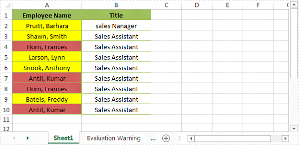
2017-12-12 09:38:16 Written by AdministratorUsing Excel conditional formatting, we can quickly find and highlight the duplicate and unique values in a selected cell range. In this article, we’re going to show you how to programmatically highlight duplicate and unique values with different colors using Spire.XLS and conditional formatting.
Detail steps:
Step 1: Initialize an object of Workbook class and Load the Excel file.
Workbook workbook = new Workbook();
workbook.LoadFromFile("Input.xlsx");
Step 2: Get the first worksheet.
Worksheet sheet = workbook.Worksheets[0];
Step 3: Use conditional formatting to highlight duplicate values in range "A2:A10" with IndianRed color.
XlsConditionalFormats xcfs1 = sheet.ConditionalFormats.Add();
xcfs1.AddRange(sheet.Range["A2:A10"]);

IConditionalFormat format1 = xcfs1.AddCondition();
format1.FormatType = ConditionalFormatType.DuplicateValues;
format1.BackColor = Color.IndianRed;
Step 4: Use conditional formatting to highlight unique values in range "A2:A10" with Yellow color.
IConditionalFormat format2 = xcfs1.AddCondition();
format2.FormatType = ConditionalFormatType.UniqueValues;
format2.BackColor = Color.Yellow;"
Step 5: Save the file.
workbook.SaveToFile("HighlightDuplicates.xlsx", ExcelVersion.Version2013);
Screenshot:
Full code:
using Spire.Xls;
using Spire.Xls.Core;
using Spire.Xls.Core.Spreadsheet.Collections;
using System.Drawing;

namespace HighlightDuplicateandUniqueValues
{
    class Program
    {
        static void Main(string[] args)
        {
            //Load the Excel file
            Workbook workbook = new Workbook();
            workbook.LoadFromFile("Input.xlsx");

            //Get the first worksheet
            Worksheet sheet = workbook.Worksheets[0];

            //Use conditional formatting to highlight duplicate values in range "A2:A10" with IndianRed color
            XlsConditionalFormats xcfs1 = sheet.ConditionalFormats.Add();
            xcfs1.AddRange(sheet.Range["A2:A10"]);

            IConditionalFormat format1 = xcfs1.AddCondition();
            format1.FormatType = ConditionalFormatType.DuplicateValues;
            format1.BackColor = Color.IndianRed;

            //Use conditional formatting to highlight unique values in range "A2:A10" with Yellow color
            IConditionalFormat format2 = xcfs1.AddCondition();
            format2.FormatType = ConditionalFormatType.UniqueValues;
            format2.BackColor = Color.Yellow;

            //Save the file
            workbook.SaveToFile("HighlightDuplicates.xlsx", ExcelVersion.Version2013);

        }
    }
}
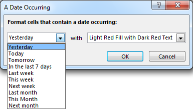
Microsoft Excel provides 10 date options, ranging from yesterday to next month (see below image) to format selected cells based on the current date. Spire.XLS supports all of these options, in this article, we’re going to show you how to conditionally format dates in Excel using Spire.XLS. If you want to highlight cells based on a date in another cell, or create rules for other dates (i.e., more than a month from the current date), you will have to create your own conditional formatting rule based on a formula.
Detail steps:
Step 1: Initialize an object of Workbook class and load the Excel file.
Workbook workbook = new Workbook();
workbook.LoadFromFile("Input.xlsx");
Step 2: Get the first worksheet.
Worksheet sheet = workbook.Worksheets[0];
Step 3: Add a condition to the used range in the worksheet.
XlsConditionalFormats xcfs1 = sheet.ConditionalFormats.Add();
xcfs1.AddRange(sheet.AllocatedRange);
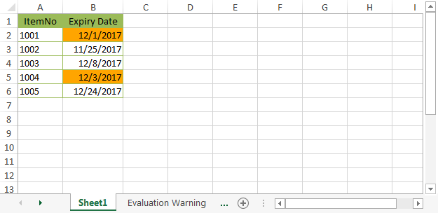
Step 4: Specify the format type of the condition as time period and set the time period as last 7 days.
IConditionalFormat format1 = xcfs1.AddTimePeriodCondition(TimePeriodType.Last7Days);
Step 5:Set the highlight color.
conditionalFormat.BackColor = Color.Orange;
Step 6:Save the file.
workbook.SaveToFile("ConditionallyFormatDates.xlsx", ExcelVersion.Version2013);
Screenshot::
Full Code:
using Spire.Xls;
using Spire.Xls.Core;
using Spire.Xls.Core.Spreadsheet.Collections;
using Spire.Xls.Core.Spreadsheet.ConditionalFormatting;
using System.Drawing;

namespace ConditionallyFormatDates
{
    class Program
    {
        static void Main(string[] args)
        {
            //Initialize an object of Workbook class
            Workbook workbook = new Workbook();

            //Load the Excel file
            workbook.LoadFromFile("Input.xlsx");

            //Get the first worksheet
            Worksheet sheet = workbook.Worksheets[0];

            //Highlight cells that contain a date occurring in the last 7 days
            XlsConditionalFormats xcfs1 = sheet.ConditionalFormats.Add();
            xcfs1.AddRange(sheet.AllocatedRange);

            IConditionalFormat conditionalFormat = xcfs1.AddTimePeriodCondition(TimePeriodType.Last7Days);
            conditionalFormat.BackColor = Color.Orange;

            //Save the file
            workbook.SaveToFile("ConditionallyFormatDates.xlsx", ExcelVersion.Version2013);
        }
    }
}
With the help of Spire.XLS, we can set the conditional format the Excel cell in C# and VB.NET. We can also use Spire.XLS to remove the conditional format from a specific cell or the entire Excel worksheet. This article will demonstrate how to remove conditional format from Excel in C#.
Firstly, view the original Excel worksheet with conditional formats:
Step 1: Create an instance of Excel workbook and load the document from file.
Workbook workbook = new Workbook();
workbook.LoadFromFile("Sample.xlsx");
Step 2: Get the first worksheet from the workbook.
Worksheet sheet = workbook.Worksheets[0];
Step 3: Remove the first conditional format.
sheet.ConditionalFormats.RemoveAt(0);
Step 4: Remove all the conditional formats from the whole Excel worksheet.
for (int i = sheet.ConditionalFormats.Count-1; i >= 0; i--)
{
sheet.ConditionalFormats.RemoveAt(i);
}
Step 5: Save the document to file.
workbook.SaveToFile("Result.xlsx", ExcelVersion.Version2010);
Remove the conditional format from a special Excel range B2:
Remove all the conditional formats from the entire Excel worksheet:
Full codes of how to remove the conditional formats from Excel worksheet:
using Spire.Xls;

namespace RemoveConditionalFormat
{
    class Program
    {
        static void Main(string[] args)
        {
            Workbook workbook = new Workbook();
            workbook.LoadFromFile("Sample.xlsx");

            Worksheet sheet = workbook.Worksheets[0];

            // Remove the first conditional format
            //sheet.ConditionalFormats.RemoveAt(0);

            // Remove all conditional formats
            for (int i = sheet.ConditionalFormats.Count-1; i >= 0; i--)
            {
                sheet.ConditionalFormats.RemoveAt(i);
            }

            workbook.SaveToFile("Result.xlsx", ExcelVersion.Version2010);
        }
    }
}
How to create a formula to apply conditional formatting in Excel in C#
2016-05-11 07:40:52 Written by KoohjiWe always use conditional formatting to highlight the cells with certain color from the whole data in the Excel worksheet. Spire.XLS also supports to create a formula to apply conditional formatting in Excel in C#. This article will show you how to apply a conditional formatting rule.
View the steps of Microsoft Excel set the conditional formatting.
Step 1: Choose the column B and then click "New Rule" under "Conditional Formatting"
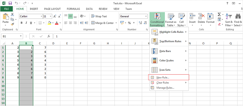
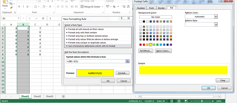
Step 2: Select the rule type, enter the rule by adding the formula and then add the highlight color for the format.
Here comes to the steps of how to set the conditional formatting rule by Spire.XLS in C#.
Step 1: Create a new excel workbook and load the document from file.
Workbook wb = new Workbook();
wb.LoadFromFile("Test.xlsx");
Step 2: Get the first worksheet and the second column from the workbook.
Worksheet sheet = wb.Worksheets[0];
CellRange range = sheet.Columns[1];
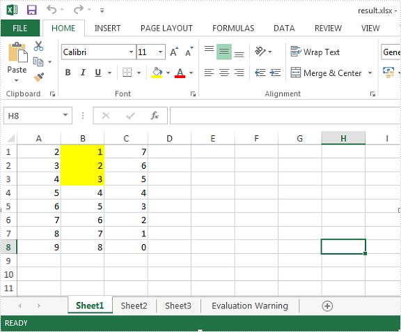
Step 3: Set the conditional formatting formula and apply the rule to the chosen cell range.
XlsConditionalFormats xcfs = sheet.ConditionalFormats.Add();
xcfs.AddRange(range);
IConditionalFormat conditional = xcfs.AddCondition();
conditional.FormatType = ConditionalFormatType.Formula;
conditional.FirstFormula = "=($B1<$C1)";
conditional.BackKnownColor = ExcelColors.Yellow;
Step 4: Save the document to file.
wb.SaveToFile("result.xlsx", ExcelVersion.Version2010);
Effective screenshot:
Full codes:
using Spire.Xls;

namespace  CreateFormula
{
    class Program
    {
        static void Main(string[] args)
        {
                Workbook wb = new Workbook();
                wb.LoadFromFile("Test.xlsx");

                Worksheet sheet = wb.Worksheets[0];
                CellRange range = sheet.Columns[1];

                XlsConditionalFormats xcfs = sheet.ConditionalFormats.Add();
                xcfs.AddRange(range);
                IConditionalFormat conditional = xcfs.AddCondition();
                conditional.FormatType = ConditionalFormatType.Formula;
                conditional.FirstFormula = "=($B1<$C1)";
                conditional.BackKnownColor = ExcelColors.Yellow;

                wb.SaveToFile("result.xlsx", ExcelVersion.Version2010);
        }
    }
}
Imports Spire.Xls

Namespace CreateFormula
  Class Program
    Private Shared Sub Main(args As String())
      Dim wb As New Workbook()
      wb.LoadFromFile("Test.xlsx")

      Dim sheet As Worksheet = wb.Worksheets(0)
      Dim range As CellRange = sheet.Columns(1)

      Dim xcfs As XlsConditionalFormats = sheet.ConditionalFormats.Add()
      xcfs.AddRange(range)
      Dim conditional As IConditionalFormat = xcfs.AddCondition()
      conditional.FormatType = ConditionalFormatType.Formula
      conditional.FirstFormula = "=($B1<$C1)"
      conditional.BackKnownColor = ExcelColors.Yellow

      wb.SaveToFile("result.xlsx", ExcelVersion.Version2010)
    End Sub
  End Class
End Namespace
By using Spire.XLS, developers can easily set the IconSetType of conditional formatting. This article will demonstrate how to set the traffic lights icons in C# with the help of Spire.XLS.
Note: Before Start, please download the latest version of Spire.XLS and add Spire.xls.dll in the bin folder as the reference of Visual Studio.
Here comes to the code snippets:
Step 1: Create a new excel document instance and get the first worksheet.
Workbook wb = new Workbook();
Worksheet sheet = wb.Worksheets[0];
Step 2: Add some data to the Excel sheet cell range and set the format for them.
sheet.Range["A1"].Text = "Traffic Lights";
sheet.Range["A2"].NumberValue = 0.95;
sheet.Range["A2"].NumberFormat = "0%";
sheet.Range["A3"].NumberValue = 0.5;
sheet.Range["A3"].NumberFormat = "0%";
sheet.Range["A4"].NumberValue = 0.1;
sheet.Range["A4"].NumberFormat = "0%";
sheet.Range["A5"].NumberValue = 0.9;
sheet.Range["A5"].NumberFormat = "0%";
sheet.Range["A6"].NumberValue = 0.7;
sheet.Range["A6"].NumberFormat = "0%";
sheet.Range["A7"].NumberValue = 0.6;
sheet.Range["A7"].NumberFormat = "0%";
Step 3: Set the height of row and width of column for Excel cell range.
sheet.AllocatedRange.RowHeight = 20;
sheet.AllocatedRange.ColumnWidth = 25;
Step 4: Add a conditional formatting of cell range and set its type to CellValue.
XlsConditionalFormats xcfs1 = sheet.ConditionalFormats.Add();
xcfs1.AddRange(sheet.AllocatedRange);
IConditionalFormat cf1 = xcfs1.AddCondition();
cf1.FormatType= ConditionalFormatType.CellValue;
cf1.FirstFormula = "300";
cf1.Operator = ComparisonOperatorType.Less;
cf1.FontColor = Color.Black;
cf1.BackColor = Color.LightSkyBlue;
Step 5: Add a conditional formatting of cell range and set its type to IconSet.
IConditionalFormat cf2 = xcfs1.AddCondition();
cf2.FormatType = ConditionalFormatType.IconSet;
cf2.IconSet.IconSetType = IconSetType.ThreeTrafficLights1;
Step 6: Save the document to file.
wb.SaveToFile("Light.xlsx", ExcelVersion.Version2010);"
Effective screenshots of the traffic lights icons set by Spire.XLS.
![]()
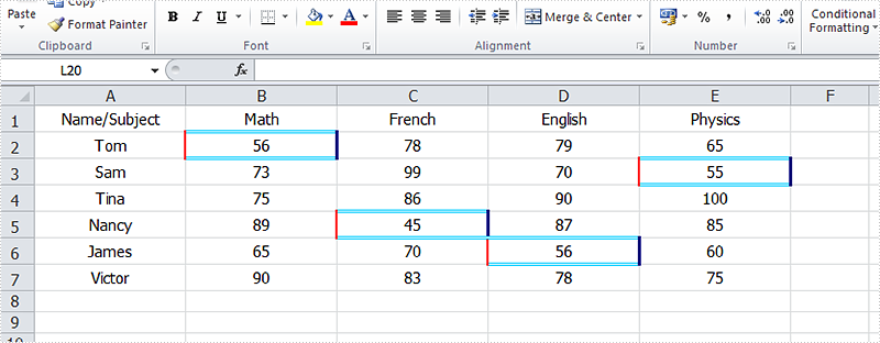
How to format cells with borders in conditional formatting
2015-08-31 01:31:47 Written by AdministratorUsing conditional formatting in Excel, we could highlight interesting cells, emphasize unusual values and visualize data with Data Bars, Color Scales and Icon Sets based on criteria. In the two articles Alternate Row Colors in Excel with Conditional Formatting and Apply Conditional Formatting to a Data Range, we have introduce the method to set fill, font, data bars, color scales and icon sets in conditional formatting using Spire.XLS. This article is going to introduce the method to format cells with borders in conditional formatting.
Note: before start, please download the latest version of Spire.XLS and add the .dll in the bin folder as the reference of Visual Studio.
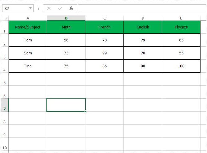
Step 1: Create a new workbook and add sample data.
            Workbook workbook = new Workbook();
            Worksheet sheet = workbook.Worksheets[0];

            sheet.Range["A1"].Value = "Name/Subject";
            sheet.Range["A2"].Value = "Tom";
            sheet.Range["A3"].Value = "Sam";
            sheet.Range["A4"].Value = "Tina";
            sheet.Range["A5"].Value = "Nancy";
            sheet.Range["A6"].Value = "James";
            sheet.Range["A7"].Value = "Victor";
            sheet.Range["B1"].Value = "Math";
            sheet.Range["C1"].Value = "French";
            sheet.Range["D1"].Value = "English";
            sheet.Range["E1"].Value = "Physics";
            sheet.Range["B2"].NumberValue = 56;
            sheet.Range["B3"].NumberValue = 73;
            sheet.Range["B4"].NumberValue = 75;
            sheet.Range["B5"].NumberValue = 89;
            sheet.Range["B6"].NumberValue = 65;
            sheet.Range["B7"].NumberValue = 90;
            sheet.Range["C2"].NumberValue = 78;
            sheet.Range["C3"].NumberValue = 99;
            sheet.Range["C4"].NumberValue = 86;
            sheet.Range["C5"].NumberValue = 45;
            sheet.Range["C6"].NumberValue = 70;
            sheet.Range["C7"].NumberValue = 83;
            sheet.Range["D2"].NumberValue = 79;
            sheet.Range["D3"].NumberValue = 70;
            sheet.Range["D4"].NumberValue = 90;
            sheet.Range["D5"].NumberValue = 87;
            sheet.Range["D6"].NumberValue = 56;
            sheet.Range["D7"].NumberValue = 78;
            sheet.Range["E2"].NumberValue = 65;
            sheet.Range["E3"].NumberValue = 55;
            sheet.Range["E4"].NumberValue = 100;
            sheet.Range["E5"].NumberValue = 85;
            sheet.Range["E6"].NumberValue = 60;
            sheet.Range["E7"].NumberValue = 75;

            sheet.AllocatedRange.RowHeight = 17;
            sheet.AllocatedRange.ColumnWidth = 17;
            sheet.AllocatedRange.VerticalAlignment = VerticalAlignType.Center;
            sheet.AllocatedRange.HorizontalAlignment = HorizontalAlignType.Center;
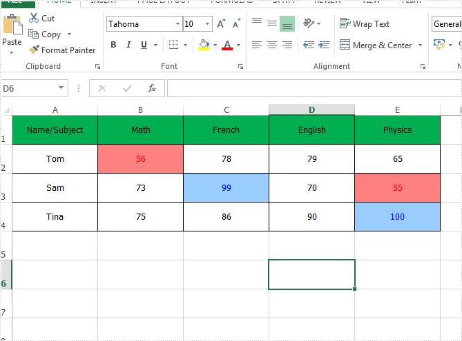
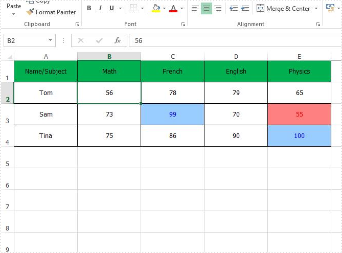
Step 2: Set the formatting rule using formula. Here the rule is the number values less than 60.
XlsConditionalFormats xcfs1 = sheet.ConditionalFormats.Add();
xcfs1.AddRange(sheet.Range["B2:E7"]);
IConditionalFormat format1 = xcfs1.AddCondition();
format1.FormatType = ConditionalFormatType.CellValue;
format1.FirstFormula = "60";
format1.Operator = ComparisonOperatorType.Less;
Step 3: Set border colors and styles for cells that match the condition.
            format1.LeftBorderColor = Color.Red;
            format1.RightBorderColor = Color.DarkBlue;
            format1.TopBorderColor = Color.DeepSkyBlue;
            format1.BottomBorderColor = Color.DeepSkyBlue;

            format1.LeftBorderStyle = LineStyleType.Medium;
            format1.RightBorderStyle = LineStyleType.Thick;
            format1.TopBorderStyle = LineStyleType.Double;
            format1.BottomBorderStyle = LineStyleType.Double;
Step 4: Save the document and launch to see effects.
            workbook.SaveToFile("sample.xlsx", ExcelVersion.Version2010);
            System.Diagnostics.Process.Start("sample.xlsx");
Effects:
Full Codes:
using Spire.Xls;
using Spire.Xls.Core;
using Spire.Xls.Core.Spreadsheet.Collections;
using System.Drawing;

namespace ApplyConditionalFormatting
{
    class Program
    {
        static void Main(string[] args)
        {
            Workbook workbook = new Workbook();
            Worksheet sheet = workbook.Worksheets[0];

            sheet.Range["A1"].Value = "Name/Subject";
            sheet.Range["A2"].Value = "Tom";
            sheet.Range["A3"].Value = "Sam";
            sheet.Range["A4"].Value = "Tina";
            sheet.Range["A5"].Value = "Nancy";
            sheet.Range["A6"].Value = "James";
            sheet.Range["A7"].Value = "Victor";
            sheet.Range["B1"].Value = "Math";
            sheet.Range["C1"].Value = "French";
            sheet.Range["D1"].Value = "English";
            sheet.Range["E1"].Value = "Physics";
            sheet.Range["B2"].NumberValue = 56;
            sheet.Range["B3"].NumberValue = 73;
            sheet.Range["B4"].NumberValue = 75;
            sheet.Range["B5"].NumberValue = 89;
            sheet.Range["B6"].NumberValue = 65;
            sheet.Range["B7"].NumberValue = 90;
            sheet.Range["C2"].NumberValue = 78;
            sheet.Range["C3"].NumberValue = 99;
            sheet.Range["C4"].NumberValue = 86;
            sheet.Range["C5"].NumberValue = 45;
            sheet.Range["C6"].NumberValue = 70;
            sheet.Range["C7"].NumberValue = 83;
            sheet.Range["D2"].NumberValue = 79;
            sheet.Range["D3"].NumberValue = 70;
            sheet.Range["D4"].NumberValue = 90;
            sheet.Range["D5"].NumberValue = 87;
            sheet.Range["D6"].NumberValue = 56;
            sheet.Range["D7"].NumberValue = 78;
            sheet.Range["E2"].NumberValue = 65;
            sheet.Range["E3"].NumberValue = 55;
            sheet.Range["E4"].NumberValue = 100;
            sheet.Range["E5"].NumberValue = 85;
            sheet.Range["E6"].NumberValue = 60;
            sheet.Range["E7"].NumberValue = 75;

            sheet.AllocatedRange.RowHeight = 17;
            sheet.AllocatedRange.ColumnWidth = 17;
            sheet.AllocatedRange.VerticalAlignment = VerticalAlignType.Center;
            sheet.AllocatedRange.HorizontalAlignment = HorizontalAlignType.Center;

            // Apply conditional formatting to the score range (B2:E7)
            XlsConditionalFormats xcfs1 = sheet.ConditionalFormats.Add();
            xcfs1.AddRange(sheet.Range["B2:E7"]);

            // Highlight cells with scores less than 60 using custom borders
            IConditionalFormat format1 = xcfs1.AddCondition();
            format1.FormatType = ConditionalFormatType.CellValue; // Compare cell values
            format1.FirstFormula = "60";
            format1.Operator = ComparisonOperatorType.Less;

            // Set border colors
            format1.LeftBorderColor = Color.Red;
            format1.RightBorderColor = Color.DarkBlue;
            format1.TopBorderColor = Color.DeepSkyBlue;
            format1.BottomBorderColor = Color.DeepSkyBlue;

            // Set border styles
            format1.LeftBorderStyle = LineStyleType.Medium;
            format1.RightBorderStyle = LineStyleType.Thick;
            format1.TopBorderStyle = LineStyleType.Double;
            format1.BottomBorderStyle = LineStyleType.Double;

            workbook.SaveToFile("sample.xlsx", ExcelVersion.Version2010);
            System.Diagnostics.Process.Start("sample.xlsx");
        }
    }
}
How to Apply Conditional Formatting to a Data Range in C#
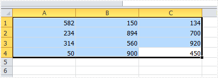
2015-03-13 07:22:54 Written by AdministratorConditional formatting in Microsoft Excel has a number of presets that enables users to apply predefined formatting such as colors, icons and data bars, to a range of cells based on the value of the cell or the value of a formula. Conditional formatting usually reveals the data trends or highlights the data that meets one or more formulas.
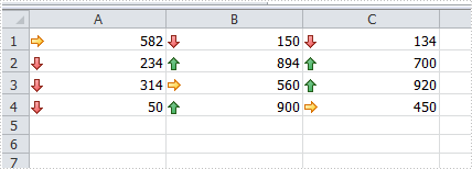
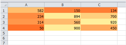
In this article, I made an example to explain how these conditional formatting types can be achieved programmatically using Spire.XLS in C#. First of all, let's see the worksheet that contains a group of data in selected range as below, we’d like see which cells’ value is bigger than 800. In order to quickly figure out similar things like this, we can create a conditional formatting rule by formula: “If the value is bigger than 800, color the cell with Red” to highlight the qualified cells.
Code Snippet for Creating Conditional Formatting Rules:
Step 1: Create a worksheet and insert data to cell range from A1 to C4.
Workbook workbook = new Workbook();
Worksheet sheet = workbook.Worksheets[0];

sheet.Range["A1"].NumberValue = 582;
sheet.Range["A2"].NumberValue = 234;
sheet.Range["A3"].NumberValue = 314;
sheet.Range["A4"].NumberValue = 50;
sheet.Range["B1"].NumberValue = 150;
sheet.Range["B2"].NumberValue = 894;
sheet.Range["B3"].NumberValue = 560;
sheet.Range["B4"].NumberValue = 900;
sheet.Range["C1"].NumberValue = 134;
sheet.Range["C2"].NumberValue = 700;
sheet.Range["C3"].NumberValue = 920;
sheet.Range["C4"].NumberValue = 450;
sheet.AllocatedRange.RowHeight = 15;
sheet.AllocatedRange.ColumnWidth = 17;
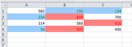
Step 2: To highlight cells based on their values, we create two conditional formatting rules: one for cells greater than 800, and another for cells less than 300.
XlsConditionalFormats xcfs1 = sheet.ConditionalFormats.Add();
xcfs1.AddRange(sheet.AllocatedRange);

IConditionalFormat cf1 = xcfs1.AddCondition();
cf1.FormatType = ConditionalFormatType.CellValue;
cf1.FirstFormula = "800";
cf1.Operator = ComparisonOperatorType.Greater;
cf1.FontColor = Color.Red;
cf1.BackColor = Color.LightSalmon;

Apply Data Bars:
IConditionalFormat cf3 = xcfs1.AddCondition();
cf3.FormatType = ConditionalFormatType.DataBar;
cf3.DataBar.BarColor = Color.CadetBlue;

Apply Icon Sets:
IConditionalFormat cf4 = xcfs1.AddCondition();
cf4.FormatType = ConditionalFormatType.IconSet;

Apply Color Scales:
IConditionalFormat cf5 = xcfs1.AddCondition();
cf5.FormatType = ConditionalFormatType.ColorScale;
Step 3: Save and launch the file
workbook.SaveToFile("sample.xlsx", ExcelVersion.Version2010);
System.Diagnostics.Process.Start("sample.xlsx");
Result:
The cells with value bigger than 800 and smaller than 300, have been highlighted with defined text color and background color.
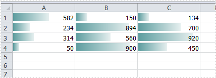
Apply the Other Three Conditional Formatting Types:
Spire.XLS also supports applying some other conditional formatting types which were predefined in MS Excel. Use the following code snippets to get more formatting effects.
Apply Data Bars:
ConditionalFormatWrapper format = sheet.AllocatedRange.ConditionalFormats.AddCondition();
format.FormatType = ConditionalFormatType.DataBar;
format.DataBar.BarColor = Color.CadetBlue;
Apply Icon Sets:
ConditionalFormatWrapper format = sheet.AllocatedRange.ConditionalFormats.AddCondition();
format.FormatType = ConditionalFormatType.IconSet;
Apply Color Scales:
ConditionalFormatWrapper format = sheet.AllocatedRange.ConditionalFormats.AddCondition();
format.FormatType = ConditionalFormatType.ColorScale;
Full Code:
using Spire.Xls;
using Spire.Xls.Core;
using Spire.Xls.Core.Spreadsheet.Collections;
using System.Drawing;

namespace ApplyConditionalFormatting
{
    class Program
    {
        static void Main(string[] args)
        {
            // Create a new workbook and get the first worksheet
            Workbook workbook = new Workbook();
            Worksheet sheet = workbook.Worksheets[0];

            // Populate sample data in cells A1:C4
            sheet.Range["A1"].NumberValue = 582;
            sheet.Range["A2"].NumberValue = 234;
            sheet.Range["A3"].NumberValue = 314;
            sheet.Range["A4"].NumberValue = 50;
            sheet.Range["B1"].NumberValue = 150;
            sheet.Range["B2"].NumberValue = 894;
            sheet.Range["B3"].NumberValue = 560;
            sheet.Range["B4"].NumberValue = 900;
            sheet.Range["C1"].NumberValue = 134;
            sheet.Range["C2"].NumberValue = 700;
            sheet.Range["C3"].NumberValue = 920;
            sheet.Range["C4"].NumberValue = 450;
            sheet.AllocatedRange.RowHeight = 15;
            sheet.AllocatedRange.ColumnWidth = 17;

            // Create a conditional formatting rule set applied to the entire used range
            XlsConditionalFormats xcfs1 = sheet.ConditionalFormats.Add();
            xcfs1.AddRange(sheet.AllocatedRange);

            // Rule 1: Highlight cells with values greater than 800 in red text and light salmon background
            IConditionalFormat cf1 = xcfs1.AddCondition();
            cf1.FormatType = ConditionalFormatType.CellValue;
            cf1.FirstFormula = "800";
            cf1.Operator = ComparisonOperatorType.Greater;
            cf1.FontColor = Color.Red;
            cf1.BackColor = Color.LightSalmon;

            // Rule 2: Highlight cells with values less than 300 in green text and light blue background
            IConditionalFormat cf2 = xcfs1.AddCondition();
            cf2.FormatType = ConditionalFormatType.CellValue;
            cf2.FirstFormula = "300";
            cf2.Operator = ComparisonOperatorType.Less;
            cf2.FontColor = Color.Green;
            cf2.BackColor = Color.LightBlue;

            //// Rule 3: Add data bars
            //IConditionalFormat cf3 = xcfs1.AddCondition();
            //cf3.FormatType = ConditionalFormatType.DataBar;
            //cf3.DataBar.BarColor = Color.CadetBlue;

            //// Rule 4: Apply icon set
            //IConditionalFormat cf4 = xcfs1.AddCondition();
            //cf4.FormatType = ConditionalFormatType.IconSet;

            //// Rule 5: Apply color scale
            //IConditionalFormat cf5 = xcfs1.AddCondition();
            //cf5.FormatType = ConditionalFormatType.ColorScale;

            workbook.SaveToFile("sample.xlsx", ExcelVersion.Version2010);
            System.Diagnostics.Process.Start("sample.xlsx");
        }
    }
}