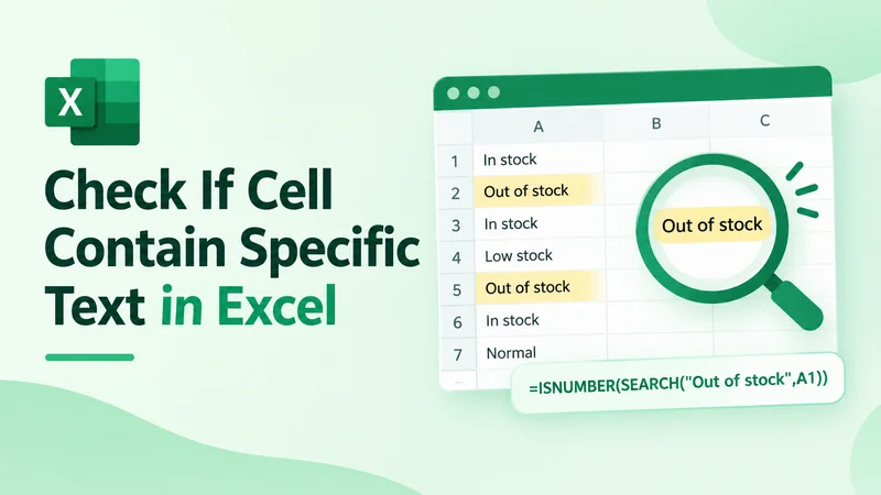
Ao trabalhar com dados do Excel, você pode precisar verificar se uma célula contém texto específico para encontrar palavras-chave, filtrar registros ou categorizar informações. Por exemplo, você pode identificar produtos marcados como fora de estoque ou realçar células que contenham termos específicos.

Este guia explica como verificar se uma célula contém texto específico no Excel usando SEARCH, FIND, COUNTIF, formatação condicional e automação com Python usando Free Spire.XLS for Python.

Verificar se as células contêm texto específico com SEARCH e ISNUMBER

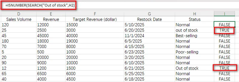
No Excel, a combinação de SEARCH e ISNUMBER é uma maneira comum de verificar se uma célula contém texto específico. Essa fórmula avalia uma célula por vez, então você precisa aplicá-la a uma coluna auxiliar e preencher a fórmula para baixo.

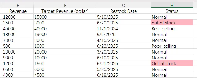
Por exemplo, se as descrições dos produtos estiverem armazenadas na coluna H, insira a fórmula em I2:

=ISNUMBER(SEARCH("Out of stock",H2))

Em seguida, copie a fórmula para baixo para aplicar a mesma verificação às linhas restantes no intervalo.

A fórmula retorna TRUE para linhas em que a célula correspondente contém out of stock e FALSE para linhas sem a palavra-chave.

Por que usar SEARCH com ISNUMBER?

A função SEARCH encontra a posição de um texto específico dentro de uma célula. Quando encontra uma correspondência, retorna a posição inicial do texto. Por exemplo, =SEARCH("stock","Out of stock") retorna 9 porque stock começa no nono caractere.

Se o texto de destino não existir, SEARCH retorna um erro #VALUE!. Ao combiná-lo com ISNUMBER, você pode converter esse resultado em um valor simples TRUE/FALSE:

• Quando SEARCH retorna um número, ISNUMBER retorna TRUE.
• Quando SEARCH retorna um erro, ISNUMBER retorna FALSE.

Esse método funciona bem quando você precisa de um resultado de correspondência claro para cada linha, como criar filtros, adicionar formatação condicional ou marcar registros para processamento posterior.

Pesquisa com diferenciação de maiúsculas e minúsculas com FIND e ISNUMBER

Em algumas situações, letras maiúsculas e minúsculas são importantes. Isso é comum ao trabalhar com códigos de produtos, identificadores internos ou categorias em que capitalizações diferentes representam valores diferentes.

A função FIND funciona de forma semelhante à SEARCH, mas realiza uma pesquisa com diferenciação de maiúsculas e minúsculas. Ao combinar FIND com ISNUMBER, você pode verificar se uma célula contém texto específico enquanto preserva as diferenças de capitalização.

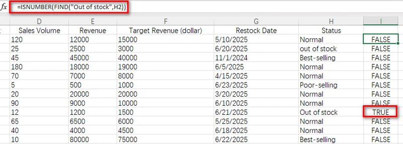
Por exemplo, suponha que uma coluna de status de produto contenha valores como "out of stock" e "Out of stock". Se você deseja identificar apenas células que usam a capitalização exata Out of stock, pode usar a seguinte fórmula em uma coluna auxiliar e aplicá-la a todo o intervalo de dados:

=ISNUMBER(FIND("Out of stock",H2))

Essa fórmula retorna TRUE quando a célula correspondente contém "Out of stock" e FALSE quando contém "out of stock" ou outro texto. Diferentemente de SEARCH, FIND distingue letras maiúsculas e minúsculas, o que a torna adequada para verificações de texto com diferenciação de maiúsculas e minúsculas.

SEARCH vs FIND

Método	Diferencia maiúsculas de minúsculas	Suporta curingas	Melhor usado para
ISNUMBER(SEARCH(...))	Não	Sim	Pesquisas gerais por palavras-chave
ISNUMBER(FIND(...))	Sim	Não	Pesquisas com diferenciação de maiúsculas e minúsculas

Verificar se a célula contém determinado texto com COUNTIF e curingas no Excel

Se você prefere uma fórmula mais curta, COUNTIF oferece uma maneira simples de verificar se uma célula contém texto específico. Esse método é útil quando você já está familiarizado com fórmulas de critérios do Excel e deseja evitar combinar várias funções.

Diferentemente de SEARCH, COUNTIF pode usar caracteres curinga, como *, para corresponder a padrões de texto. Isso o torna conveniente para verificações básicas de palavras-chave.

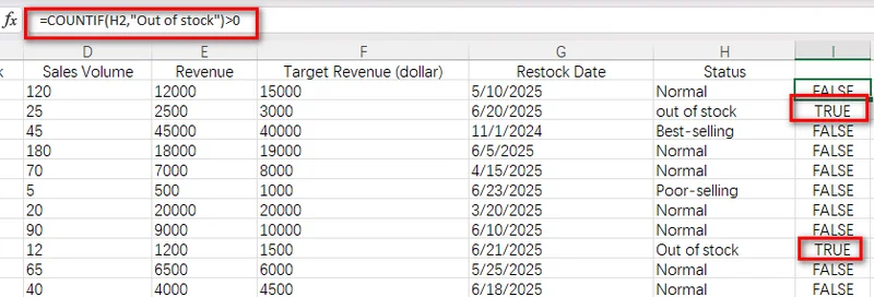
Insira a seguinte fórmula em uma célula da coluna auxiliar:

=COUNTIF(H2,"Out of stock")>0

A fórmula retorna TRUE quando a célula contém "out of stock" e FALSE quando o texto especificado não é encontrado.

Como o asterisco (*) funciona

Em COUNTIF, o asterisco (*) é um curinga que representa qualquer número de caracteres. Ao colocar um asterisco antes e depois do texto de destino, você permite que o Excel corresponda à palavra-chave onde quer que ela apareça dentro de uma célula.

Por exemplo, usar stock como padrão de pesquisa corresponderá a células que contenham apenas stock, bem como a frases mais longas, como "out of stock" ou "low stock warning". Isso ocorre porque os caracteres curinga permitem que qualquer texto apareça antes ou depois da palavra-chave.

Dica: Se você precisa contar células que contêm texto em vez de apenas verificar uma correspondência, consulte nosso guia sobre contar células com texto no Excel.

Verificar várias palavras-chave com lógica OR no Excel

Em alguns casos, você pode precisar verificar se uma célula contém uma entre várias palavras-chave. Por exemplo, ao analisar status de produtos, você pode querer identificar itens que estão fora de estoque ou têm baixo desempenho de vendas. A função OR permite combinar várias verificações de texto em uma única fórmula. Semelhante aos métodos anteriores.

Insira a seguinte fórmula em uma célula de uma coluna auxiliar:

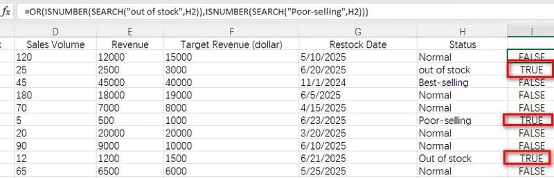
=OR(ISNUMBER(SEARCH("out of stock",H2)),ISNUMBER(SEARCH("Poor-selling",H2)))

A fórmula retorna TRUE quando o status correspondente contém "out of stock" ou "Poor-selling". Ela retorna FALSE para status normais ou outros valores.

Realçar células que contêm texto específico com formatação condicional

Usar uma coluna auxiliar é uma maneira prática de verificar se as células contêm texto específico, mas exige uma coluna adicional para exibir os resultados. Se você deseja tornar os registros correspondentes mais visíveis sem alterar a estrutura dos dados, a Formatação Condicional é uma opção melhor.

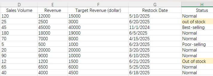
Com a formatação condicional, o Excel pode realçar automaticamente células que atendem a uma regra específica. Ao usar uma fórmula baseada em SEARCH, você pode realçar células correspondentes sempre que os dados forem alterados.

Siga estas etapas para aplicar a formatação condicional:

• Etapa 1: Selecione o intervalo de destino, como H2:H15.
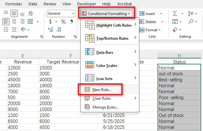
• Etapa 2: Vá para Página Inicial > Formatação Condicional > Nova Regra.

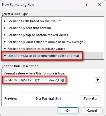
• Etapa 3: Selecione Usar uma fórmula para determinar quais células devem ser formatadas.
• Etapa 4: Insira a fórmula =ISNUMBER(SEARCH("Out of stock",H2)).

• Etapa 5: Clique em Formatar..., escolha um estilo de formatação e clique em OK para aplicar a regra.

Verificar automaticamente se uma célula contém determinado texto com Python

Métodos baseados em fórmulas funcionam bem ao processar planilhas individuais, mas adicionar fórmulas ou regras de formatação manualmente pode se tornar ineficiente ao lidar com relatórios recorrentes ou grandes quantidades de arquivos do Excel.

Em fluxos de trabalho automatizados, desenvolvedores podem usar Python para aplicar a mesma lógica de verificação de texto programaticamente. Com o Free Spire.XLS for Python, você pode criar, editar e formatar pastas de trabalho do Excel sem depender do Microsoft Excel.

O que é Free Spire.XLS for Python?

Free Spire.XLS for Python é uma biblioteca Python para trabalhar com pastas de trabalho do Excel. Ela oferece suporte a operações comuns de planilha, como criar arquivos, ler e editar planilhas, aplicar fórmulas, adicionar formatação condicional e converter documentos do Excel.

Usando esta biblioteca, desenvolvedores podem automatizar tarefas repetitivas de planilha, como aplicar regras de formatação baseadas em texto em vários relatórios.

Implementação passo a passo em Python

O exemplo a seguir mostra como carregar uma pasta de trabalho do Excel e aplicar automaticamente uma regra de formatação condicional com base na presença de uma frase específica nas células.

Etapa 1: Instalar a biblioteca

Instale o pacote usando pip:

pip install Spire.Xls.Free

Etapa 2: Aplicar formatação condicional com Python

O script a seguir carrega um arquivo do Excel e realça células que contêm out of stock.

from spire.xls import Workbook, Color

file_path = "input/sales report.xlsx"
output_path = "output/Highlighted.xlsx"

# Load the Excel workbook
workbook = Workbook()
workbook.LoadFromFile(file_path)
sheet = workbook.Worksheets[0]

# Target the desired cell range
range_data = sheet.Range["H2:H15"]

# Add an expression-based conditional formatting rule
rule = range_data.ConditionalFormats.AddCondition()
rule.FormatType = ConditionalFormatType.Formula
rule.FirstFormula = '=ISNUMBER(SEARCH("Out of stock", H2))'

# Apply background color for matching cells
rule.BackColor = Color.get_LightPink()

# Save output and release resources
workbook.SaveToFile(output_path)
workbook.Dispose()

Armadilhas comuns e perguntas frequentes

P1: Por que minha fórmula retorna um erro #VALUE!?

Se você usar SEARCH ou FIND sozinho e o texto especificado não existir na célula, o Excel retorna um erro #VALUE!. Se você precisar determinar se o texto existe, use ISNUMBER para converter o resultado da pesquisa em TRUE ou FALSE.

P2: Qual é a diferença entre verificar texto específico e ISTEXT()?

A função ISTEXT verifica se uma célula contém dados de texto, então ela pode ajudar a distinguir valores de texto de números, datas e outros tipos de dados. Por exemplo, =ISTEXT(A1) retorna TRUE quando a célula contém texto e FALSE quando contém um número ou outro tipo de dados.

No entanto, ISTEXT não consegue verificar se uma célula contém texto específico. Se você precisar pesquisar uma palavra ou frase específica, use SEARCH, FIND ou COUNTIF em vez disso.

P3: Como posso verificar se uma célula contém texto parcial?

Para verificar se uma célula contém parte de uma cadeia de texto mais longa, use SEARCH com ISNUMBER ou COUNTIF com curingas. Por exemplo, =ISNUMBER(SEARCH("stock",A1)) retorna TRUE quando a célula contém stock em qualquer lugar do texto, incluindo frases como "out of stock" ou "low stock". Você também pode usar =COUNTIF(A1,"stock")>0 para uma fórmula mais curta baseada em curinga.

Para concluir

Verificar se uma célula contém texto específico é uma tarefa comum no processamento de dados do Excel. Na maioria dos casos, ISNUMBER(SEARCH()) oferece uma solução flexível, enquanto FIND() é útil quando letras maiúsculas e minúsculas precisam ser diferenciadas. Se você prefere uma fórmula mais curta, COUNTIF() oferece uma abordagem simples baseada em curinga.

Para fluxos de trabalho recorrentes com planilhas, a automação em Python com Free Spire.XLS for Python pode ajudar a aplicar as mesmas regras de verificação de texto e formatação programaticamente, reduzindo o trabalho manual repetitivo.

---

Leia também:

• Como comparar duas colunas no Excel – 7 métodos fáceis
• Realçar duplicatas no Excel: 4 métodos fáceis
• Limpar ou remover filtros no Excel: 6 maneiras (manual e automatizada)
• Classificar dados no Excel: 5 métodos simples e avançados explicados

Excel 데이터로 작업하다 보면 키워드를 찾거나 레코드를 필터링하거나 정보를 분류하기 위해 셀에 특정 텍스트가 포함되어 있는지 확인해야 할 때가 있습니다. 예를 들어 재고 없음으로 표시된 제품을 식별하거나 특정 용어가 포함된 셀을 강조 표시할 수 있습니다.

이 가이드에서는 SEARCH, FIND, COUNTIF, 조건부 서식, 그리고 Free Spire.XLS for Python을 사용한 Python 자동화를 활용하여 Excel에서 셀에 특정 텍스트가 포함되어 있는지 확인하는 방법을 설명합니다.

SEARCH와 ISNUMBER로 셀에 특정 텍스트가 포함되어 있는지 확인하기

Excel에서는 SEARCH와 ISNUMBER의 조합이 셀에 특정 텍스트가 포함되어 있는지 확인하는 일반적인 방법입니다. 이 수식은 한 번에 하나의 셀만 평가하므로 보조 열에 적용하고 수식을 아래로 채워야 합니다.

예를 들어 제품 설명이 H열에 저장되어 있다면 I2 셀에 수식을 입력합니다:

=ISNUMBER(SEARCH("Out of stock",H2))

그런 다음 수식을 아래로 복사하여 범위의 나머지 행에도 동일한 검사를 적용합니다.

이 수식은 해당 셀에 out of stock이 포함된 행에는 TRUE를, 키워드가 없는 행에는 FALSE를 반환합니다.

SEARCH를 ISNUMBER와 함께 사용하는 이유는?

SEARCH 함수는 셀 내에서 특정 텍스트의 위치를 찾습니다. 일치하는 항목을 찾으면 텍스트의 시작 위치를 반환합니다. 예를 들어 =SEARCH("stock","Out of stock")은 stock이 9번째 문자에서 시작하므로 9를 반환합니다.

대상 텍스트가 없으면 SEARCH는 #VALUE! 오류를 반환합니다. 이를 ISNUMBER와 결합하면 이 결과를 단순한 TRUE/FALSE 값으로 변환할 수 있습니다:

• SEARCH가 숫자를 반환하면 ISNUMBER는 TRUE를 반환합니다.
• SEARCH가 오류를 반환하면 ISNUMBER는 FALSE를 반환합니다.

이 방법은 필터를 만들거나, 조건부 서식을 추가하거나, 추가 처리를 위해 레코드를 표시하는 등 각 행에 대해 명확한 일치 결과가 필요할 때 유용합니다.

FIND와 ISNUMBER로 대소문자를 구분하여 검색하기

어떤 상황에서는 대문자와 소문자가 중요합니다. 이는 서로 다른 대소문자가 서로 다른 값을 나타내는 제품 코드, 내부 식별자 또는 카테고리를 다룰 때 흔히 발생합니다.

FIND 함수는 SEARCH와 유사하게 작동하지만 대소문자를 구분하여 검색합니다. FIND를 ISNUMBER와 결합하면 대소문자 차이를 유지하면서 셀에 특정 텍스트가 포함되어 있는지 확인할 수 있습니다.

예를 들어 제품 상태 열에 "out of stock"과 "Out of stock" 같은 값이 포함되어 있다고 가정해 보겠습니다. 정확히 Out of stock 대소문자를 사용하는 셀만 식별하려면 보조 열에 다음 수식을 사용하여 전체 데이터 범위에 적용합니다:

=ISNUMBER(FIND("Out of stock",H2))

이 수식은 해당 셀에 "Out of stock"이 포함되어 있으면 TRUE를, "out of stock"이나 다른 텍스트가 포함되어 있으면 FALSE를 반환합니다. SEARCH와 달리 FIND는 대문자와 소문자를 구분하므로 대소문자를 구분하는 텍스트 검사에 적합합니다.

SEARCH vs FIND

방법	대소문자 구분	와일드카드 지원	최적 사용 사례
ISNUMBER(SEARCH(...))	아니요	예	일반적인 키워드 검색
ISNUMBER(FIND(...))	예	아니요	대소문자를 구분하는 검색

Excel에서 COUNTIF와 와일드카드로 셀에 특정 텍스트가 포함되어 있는지 확인하기

더 짧은 수식을 선호한다면 COUNTIF가 셀에 특정 텍스트가 포함되어 있는지 확인하는 간단한 방법을 제공합니다. 이 방법은 이미 Excel 조건 수식에 익숙하고 여러 함수를 결합하는 것을 피하고 싶을 때 유용합니다.

SEARCH와 달리 COUNTIF는 *와 같은 와일드카드 문자를 사용하여 텍스트 패턴을 일치시킬 수 있습니다. 따라서 기본적인 키워드 검사에 편리합니다.

보조 열의 셀에 다음 수식을 입력합니다:

=COUNTIF(H2,"Out of stock")>0

이 수식은 셀에 "out of stock"이 포함되어 있으면 TRUE를, 지정한 텍스트가 없으면 FALSE를 반환합니다.

별표(*)의 작동 방식

COUNTIF에서 별표(*)는 임의 개수의 문자를 나타내는 와일드카드입니다. 대상 텍스트 앞뒤에 별표를 배치하면 Excel이 셀 안 어디에 있든 키워드를 일치시킬 수 있습니다.

예를 들어 stock을 검색 패턴으로 사용하면 stock만 포함된 셀은 물론 "out of stock"이나 "low stock warning"과 같은 더 긴 문구가 포함된 셀도 일치합니다. 와일드카드 문자를 사용하면 키워드 앞뒤에 어떤 텍스트든 올 수 있기 때문입니다.

팁: 단순히 일치 여부를 확인하는 대신 텍스트가 포함된 셀의 개수를 세야 한다면, Excel에서 텍스트가 포함된 셀 개수 세기 가이드를 참고하세요.

Excel에서 OR 논리로 여러 키워드 확인하기

경우에 따라 셀에 여러 키워드 중 하나가 포함되어 있는지 확인해야 할 수 있습니다. 예를 들어 제품 상태를 분석할 때 재고가 없거나 판매 실적이 저조한 항목을 식별하고 싶을 수 있습니다. OR 함수를 사용하면 하나의 수식에서 여러 텍스트 검사를 결합할 수 있습니다. 앞의 방법들과 유사합니다.

보조 열의 셀에 다음 수식을 입력합니다:

=OR(ISNUMBER(SEARCH("out of stock",H2)),ISNUMBER(SEARCH("Poor-selling",H2)))

이 수식은 해당 상태에 "out of stock" 또는 "Poor-selling"이 포함되어 있으면 TRUE를 반환합니다. 정상 상태나 다른 값에 대해서는 FALSE를 반환합니다.

조건부 서식으로 특정 텍스트가 포함된 셀 강조하기

보조 열을 사용하는 것은 셀에 특정 텍스트가 포함되어 있는지 확인하는 실용적인 방법이지만, 결과를 표시할 추가 열이 필요합니다. 데이터 구조를 변경하지 않고 일치하는 레코드를 더 잘 보이게 하고 싶다면 조건부 서식이 더 나은 선택입니다.

조건부 서식을 사용하면 Excel에서 특정 규칙을 충족하는 셀을 자동으로 강조 표시할 수 있습니다. SEARCH를 기반으로 한 수식을 사용하면 데이터가 변경될 때마다 일치하는 셀을 강조 표시할 수 있습니다.

조건부 서식을 적용하려면 다음 단계를 따르세요:

• 1단계: H2:H15와 같은 대상 범위를 선택합니다.
• 2단계: 홈 > 조건부 서식 > 새 규칙으로 이동합니다.

• 3단계: 수식을 사용하여 서식을 지정할 셀 결정을 선택합니다.
• 4단계: =ISNUMBER(SEARCH("Out of stock",H2)) 수식을 입력합니다.

• 5단계: 서식...을 클릭하고 서식 스타일을 선택한 다음 확인을 클릭하여 규칙을 적용합니다.

Python으로 셀에 특정 텍스트가 포함되어 있는지 자동으로 확인하기

수식 기반 방법은 개별 스프레드시트를 처리할 때는 잘 작동하지만, 반복되는 보고서나 많은 수의 Excel 파일을 처리할 때 수식이나 서식 규칙을 수동으로 추가하는 것은 비효율적일 수 있습니다.

자동화된 워크플로에서는 개발자가 Python을 사용하여 동일한 텍스트 확인 로직을 프로그래밍 방식으로 적용할 수 있습니다. Free Spire.XLS for Python을 사용하면 Microsoft Excel에 의존하지 않고 Excel 통합 문서를 만들고, 편집하고, 서식을 지정할 수 있습니다.

Free Spire.XLS for Python이란?

Free Spire.XLS for Python은 Excel 통합 문서 작업을 위한 Python 라이브러리입니다. 파일 생성, 워크시트 읽기 및 편집, 수식 적용, 조건부 서식 추가, Excel 문서 변환 등 일반적인 스프레드시트 작업을 지원합니다.

이 라이브러리를 사용하면 개발자가 여러 보고서에 텍스트 기반 서식 규칙을 적용하는 등 반복적인 스프레드시트 작업을 자동화할 수 있습니다.

단계별 Python 구현

다음 예제에서는 Excel 통합 문서를 로드하고 셀에 특정 문구가 포함되어 있는지 여부에 따라 조건부 서식 규칙을 자동으로 적용하는 방법을 보여줍니다.

1단계: 라이브러리 설치

pip를 사용하여 패키지를 설치합니다:

pip install Spire.Xls.Free

2단계: Python으로 조건부 서식 적용

다음 스크립트는 Excel 파일을 로드하고 out of stock이 포함된 셀을 강조 표시합니다.

from spire.xls import Workbook, Color

file_path = "input/sales report.xlsx"
output_path = "output/Highlighted.xlsx"

# Load the Excel workbook
workbook = Workbook()
workbook.LoadFromFile(file_path)
sheet = workbook.Worksheets[0]

# Target the desired cell range
range_data = sheet.Range["H2:H15"]

# Add an expression-based conditional formatting rule
rule = range_data.ConditionalFormats.AddCondition()
rule.FormatType = ConditionalFormatType.Formula
rule.FirstFormula = '=ISNUMBER(SEARCH("Out of stock", H2))'

# Apply background color for matching cells
rule.BackColor = Color.get_LightPink()

# Save output and release resources
workbook.SaveToFile(output_path)
workbook.Dispose()

자주 발생하는 실수와 FAQ

Q1: 수식이 #VALUE! 오류를 반환하는 이유는?

SEARCH나 FIND를 단독으로 사용했는데 셀에 지정한 텍스트가 없으면 Excel은 #VALUE! 오류를 반환합니다. 텍스트 존재 여부를 판단해야 한다면 ISNUMBER를 사용하여 검색 결과를 TRUE 또는 FALSE로 변환하세요.

Q2: 특정 텍스트 확인과 ISTEXT()의 차이점은?

ISTEXT 함수는 셀에 텍스트 데이터가 포함되어 있는지 확인하므로 텍스트 값과 숫자, 날짜 및 기타 데이터 유형을 구분하는 데 도움이 됩니다. 예를 들어 =ISTEXT(A1)은 셀에 텍스트가 포함되어 있으면 TRUE를, 숫자나 다른 데이터 유형이 포함되어 있으면 FALSE를 반환합니다.

그러나 ISTEXT는 셀에 특정 텍스트가 포함되어 있는지 확인할 수 없습니다. 특정 단어나 문구를 검색해야 한다면 대신 SEARCH, FIND 또는 COUNTIF를 사용하세요.

Q3: 셀에 부분 텍스트가 포함되어 있는지 어떻게 확인할 수 있나요?

셀에 더 긴 텍스트 문자열의 일부가 포함되어 있는지 확인하려면 ISNUMBER와 함께 SEARCH를 사용하거나 와일드카드와 함께 COUNTIF를 사용하세요. 예를 들어 =ISNUMBER(SEARCH("stock",A1))은 셀 텍스트 어디에든 stock이 포함되어 있으면(예: "out of stock" 또는 "low stock"과 같은 문구) TRUE를 반환합니다. 더 짧은 와일드카드 기반 수식으로 =COUNTIF(A1,"stock")>0을 사용할 수도 있습니다.

마무리

셀에 특정 텍스트가 포함되어 있는지 확인하는 것은 Excel 데이터 처리에서 흔한 작업입니다. 대부분의 경우 ISNUMBER(SEARCH())가 유연한 해결책을 제공하며, FIND()는 대문자와 소문자를 구분해야 할 때 유용합니다. 더 짧은 수식을 선호한다면 COUNTIF()가 간단한 와일드카드 기반 접근 방식을 제공합니다.

반복되는 스프레드시트 워크플로의 경우 Free Spire.XLS for Python을 사용한 Python 자동화를 통해 동일한 텍스트 확인 및 서식 규칙을 프로그래밍 방식으로 적용하여 반복적인 수작업을 줄일 수 있습니다.

---

함께 읽어보세요:

• Excel에서 두 열을 비교하는 방법 – 7가지 쉬운 방법
• Excel에서 중복 항목 강조 표시: 4가지 쉬운 방법
• Excel에서 필터 지우기 또는 제거하기: 6가지 방법 (수동 및 자동)
• Excel에서 데이터 정렬하기: 5가지 간단하고 고급스러운 방법 설명

Quando si lavora con i dati di Excel, potrebbe essere necessario verificare se una cella contiene un testo specifico per trovare parole chiave, filtrare record o categorizzare informazioni. Ad esempio, è possibile identificare i prodotti contrassegnati come esauriti o evidenziare le celle che contengono termini specifici.

Questa guida spiega come verificare se una cella contiene un testo specifico in Excel utilizzando SEARCH, FIND, COUNTIF, la formattazione condizionale e l'automazione con Python tramite Free Spire.XLS for Python.

Verificare se le celle contengono un testo specifico con SEARCH e ISNUMBER

In Excel, la combinazione di SEARCH e ISNUMBER è un modo comune per verificare se una cella contiene un testo specifico. Questa formula valuta una cella alla volta, quindi è necessario applicarla a una colonna di supporto e copiarla verso il basso.

Ad esempio, se le descrizioni dei prodotti sono memorizzate nella colonna H, inserisci la formula in I2:

=ISNUMBER(SEARCH("Out of stock",H2))

Poi copia la formula verso il basso per applicare la stessa verifica alle righe rimanenti dell'intervallo.

La formula restituisce TRUE per le righe in cui la cella corrispondente contiene out of stock e FALSE per le righe senza la parola chiave.

Perché usare SEARCH con ISNUMBER?

La funzione SEARCH trova la posizione di un testo specifico all'interno di una cella. Quando trova una corrispondenza, restituisce la posizione iniziale del testo. Ad esempio, =SEARCH("stock","Out of stock") restituisce 9 perché stock inizia dal nono carattere.

Se il testo cercato non esiste, SEARCH restituisce un errore #VALUE!. Combinandola con ISNUMBER, è possibile convertire questo risultato in un semplice valore TRUE/FALSE:

• Quando SEARCH restituisce un numero, ISNUMBER restituisce TRUE.
• Quando SEARCH restituisce un errore, ISNUMBER restituisce FALSE.

Questo metodo funziona bene quando è necessario un risultato di corrispondenza chiaro per ogni riga, ad esempio per creare filtri, aggiungere la formattazione condizionale o contrassegnare i record per ulteriori elaborazioni.

Ricerca con distinzione tra maiuscole e minuscole con FIND e ISNUMBER

In alcune situazioni, le lettere maiuscole e minuscole sono importanti. Ciò è comune quando si lavora con codici prodotto, identificatori interni o categorie in cui una diversa capitalizzazione rappresenta valori diversi.

La funzione FIND funziona in modo simile a SEARCH, ma esegue una ricerca con distinzione tra maiuscole e minuscole. Combinando FIND con ISNUMBER, è possibile verificare se una cella contiene un testo specifico preservando le differenze di capitalizzazione.

Ad esempio, supponiamo che una colonna di stato del prodotto contenga valori come "out of stock" e "Out of stock". Se si desidera identificare solo le celle che utilizzano la capitalizzazione esatta Out of stock, è possibile utilizzare la seguente formula in una colonna di supporto e applicarla all'intero intervallo di dati:

=ISNUMBER(FIND("Out of stock",H2))

Questa formula restituisce TRUE quando la cella corrispondente contiene "Out of stock" e FALSE quando contiene "out of stock" o altro testo. A differenza di SEARCH, FIND distingue le lettere maiuscole dalle minuscole, rendendola adatta alle verifiche di testo con distinzione tra maiuscole e minuscole.

SEARCH vs FIND

Metodo	Distingue maiuscole/minuscole	Supporta i caratteri jolly	Ideale per
ISNUMBER(SEARCH(...))	No	Sì	Ricerche generiche di parole chiave
ISNUMBER(FIND(...))	Sì	No	Ricerche con distinzione tra maiuscole e minuscole

Verificare se una cella contiene un determinato testo con COUNTIF e i caratteri jolly in Excel

Se preferisci una formula più breve, COUNTIF offre un modo semplice per verificare se una cella contiene un testo specifico. Questo metodo è utile quando hai già familiarità con le formule di criterio di Excel e desideri evitare di combinare più funzioni.

A differenza di SEARCH, COUNTIF può utilizzare caratteri jolly come * per trovare corrispondenze con schemi di testo. Questo lo rende comodo per verifiche di base delle parole chiave.

Inserisci la seguente formula in una cella della colonna di supporto:

=COUNTIF(H2,"Out of stock")>0

La formula restituisce TRUE quando la cella contiene "out of stock" e FALSE quando il testo specificato non viene trovato.

Come funziona l'asterisco (*)

In COUNTIF, l'asterisco (*) è un carattere jolly che rappresenta un numero qualsiasi di caratteri. Inserendo un asterisco prima e dopo il testo cercato, consenti a Excel di trovare la parola chiave ovunque essa compaia all'interno di una cella.

Ad esempio, utilizzando stock come schema di ricerca si troveranno corrispondenze con celle che contengono solo stock e anche con frasi più lunghe come "out of stock" o "low stock warning". Questo perché i caratteri jolly consentono la presenza di qualsiasi testo prima o dopo la parola chiave.

Suggerimento: se devi contare le celle che contengono testo invece di verificare semplicemente una corrispondenza, consulta la nostra guida sul conteggio delle celle con testo in Excel.

Verificare più parole chiave con la logica OR in Excel

In alcuni casi, potrebbe essere necessario verificare se una cella contiene una tra diverse parole chiave. Ad esempio, analizzando gli stati dei prodotti, potresti voler identificare gli articoli che sono esauriti oppure che hanno scarse prestazioni di vendita. La funzione OR ti consente di combinare più verifiche di testo in un'unica formula. In modo simile ai metodi precedenti.

Inserisci la seguente formula in una cella di una colonna di supporto:

=OR(ISNUMBER(SEARCH("out of stock",H2)),ISNUMBER(SEARCH("Poor-selling",H2)))

La formula restituisce TRUE quando lo stato corrispondente contiene "out of stock" oppure "Poor-selling". Restituisce FALSE per stati normali o altri valori.

Evidenziare le celle che contengono un testo specifico con la formattazione condizionale

Utilizzare una colonna di supporto è un modo pratico per verificare se le celle contengono un testo specifico, ma richiede una colonna aggiuntiva per visualizzare i risultati. Se desideri rendere più visibili i record corrispondenti senza modificare la struttura dei dati, la formattazione condizionale è un'opzione migliore.

Con la formattazione condizionale, Excel può evidenziare automaticamente le celle che soddisfano una regola specifica. Utilizzando una formula basata su SEARCH, puoi evidenziare le celle corrispondenti ogni volta che i dati cambiano.

Segui questi passaggi per applicare la formattazione condizionale:

• Passaggio 1: Seleziona l'intervallo di destinazione, ad esempio H2:H15.
• Passaggio 2: Vai a Home > Formattazione condizionale > Nuova regola.

• Passaggio 3: Seleziona Utilizza una formula per determinare le celle da formattare.
• Passaggio 4: Inserisci la formula =ISNUMBER(SEARCH("Out of stock",H2)).

• Passaggio 5: Fai clic su Formato..., scegli uno stile di formattazione e poi fai clic su OK per applicare la regola.

Verificare automaticamente se una cella contiene un determinato testo con Python

I metodi basati su formule funzionano bene quando si elaborano singoli fogli di calcolo, ma aggiungere manualmente formule o regole di formattazione può diventare inefficiente quando si gestiscono report ricorrenti o un numero elevato di file Excel.

Nei flussi di lavoro automatizzati, gli sviluppatori possono utilizzare Python per applicare la stessa logica di verifica del testo in modo programmatico. Con Free Spire.XLS for Python, puoi creare, modificare e formattare cartelle di lavoro Excel senza dipendere da Microsoft Excel.

Che cos'è Free Spire.XLS for Python?

Free Spire.XLS for Python è una libreria Python per lavorare con cartelle di lavoro Excel. Supporta operazioni comuni sui fogli di calcolo come la creazione di file, la lettura e la modifica di fogli di lavoro, l'applicazione di formule, l'aggiunta della formattazione condizionale e la conversione di documenti Excel.

Utilizzando questa libreria, gli sviluppatori possono automatizzare attività ripetitive sui fogli di calcolo, come l'applicazione di regole di formattazione basate sul testo in più report.

Implementazione Python passo dopo passo

L'esempio seguente mostra come caricare una cartella di lavoro Excel e applicare automaticamente una regola di formattazione condizionale in base alla presenza di una frase specifica nelle celle.

Passaggio 1: installare la libreria

Installa il pacchetto utilizzando pip:

pip install Spire.Xls.Free

Passaggio 2: applicare la formattazione condizionale con Python

Il seguente script carica un file Excel ed evidenzia le celle che contengono out of stock.

from spire.xls import Workbook, Color

file_path = "input/sales report.xlsx"
output_path = "output/Highlighted.xlsx"

# Load the Excel workbook
workbook = Workbook()
workbook.LoadFromFile(file_path)
sheet = workbook.Worksheets[0]

# Target the desired cell range
range_data = sheet.Range["H2:H15"]

# Add an expression-based conditional formatting rule
rule = range_data.ConditionalFormats.AddCondition()
rule.FormatType = ConditionalFormatType.Formula
rule.FirstFormula = '=ISNUMBER(SEARCH("Out of stock", H2))'

# Apply background color for matching cells
rule.BackColor = Color.get_LightPink()

# Save output and release resources
workbook.SaveToFile(output_path)
workbook.Dispose()

Errori comuni e FAQ

D1: Perché la mia formula restituisce un errore #VALUE!?

Se utilizzi SEARCH o FIND da sola e il testo specificato non esiste nella cella, Excel restituisce un errore #VALUE!. Se devi determinare se il testo esiste, usa ISNUMBER per convertire il risultato della ricerca in TRUE o FALSE.

D2: Qual è la differenza tra la verifica di un testo specifico e ISTEXT()?

La funzione ISTEXT verifica se una cella contiene dati di testo, quindi può aiutare a distinguere i valori di testo da numeri, date e altri tipi di dati. Ad esempio, =ISTEXT(A1) restituisce TRUE quando la cella contiene testo e FALSE quando contiene un numero o un altro tipo di dati.

Tuttavia, ISTEXT non può verificare se una cella contiene un testo specifico. Se devi cercare una parola o una frase particolare, usa invece SEARCH, FIND o COUNTIF.

D3: Come posso verificare se una cella contiene un testo parziale?

Per verificare se una cella contiene parte di una stringa di testo più lunga, usa SEARCH con ISNUMBER oppure COUNTIF con i caratteri jolly. Ad esempio, =ISNUMBER(SEARCH("stock",A1)) restituisce TRUE quando la cella contiene stock in qualsiasi punto del suo testo, comprese frasi come "out of stock" o "low stock". Puoi anche usare =COUNTIF(A1,"stock")>0 per una formula più breve basata sui caratteri jolly.

Conclusione

Verificare se una cella contiene un testo specifico è un'operazione comune nell'elaborazione dei dati di Excel. Nella maggior parte dei casi, ISNUMBER(SEARCH()) offre una soluzione flessibile, mentre FIND() è utile quando è necessario distinguere le lettere maiuscole dalle minuscole. Se preferisci una formula più breve, COUNTIF() offre un semplice approccio basato sui caratteri jolly.

Per i flussi di lavoro ricorrenti sui fogli di calcolo, l'automazione con Python tramite Free Spire.XLS for Python può aiutare ad applicare le stesse regole di verifica del testo e di formattazione in modo programmatico, riducendo il lavoro manuale ripetitivo.

---

Leggi anche:

• Come confrontare due colonne in Excel – 7 metodi semplici
• Evidenziare i duplicati in Excel: 4 metodi semplici
• Cancellare o rimuovere i filtri in Excel: 6 modi (manuale e automatizzato)
• Ordinare i dati in Excel: 5 metodi semplici e avanzati spiegati

Lorsque vous travaillez avec des données Excel, vous pouvez avoir besoin de vérifier si une cellule contient un texte spécifique pour trouver des mots-clés, filtrer des enregistrements ou catégoriser des informations. Par exemple, vous pouvez identifier des produits marqués comme en rupture de stock ou mettre en surbrillance des cellules contenant des termes spécifiques.

Ce guide explique comment vérifier si une cellule contient un texte spécifique dans Excel à l'aide de SEARCH, FIND, COUNTIF, de la mise en forme conditionnelle et de l'automatisation Python avec Free Spire.XLS pour Python.

Vérifier si les cellules contiennent un texte spécifique avec SEARCH et ISNUMBER

Dans Excel, la combinaison de SEARCH et ISNUMBER est un moyen courant de vérifier si une cellule contient un texte spécifique. Cette formule évalue une cellule à la fois, vous devez donc l'appliquer à une colonne d'assistance et remplir la formule vers le bas.

Par exemple, si les descriptions de produits sont stockées dans la colonne H, saisissez la formule dans I2 :

=ISNUMBER(SEARCH("Out of stock",H2))

Copiez ensuite la formule vers le bas pour appliquer la même vérification aux lignes restantes de la plage.

La formule renvoie TRUE pour les lignes où la cellule correspondante contient « out of stock » et FALSE pour les lignes sans le mot-clé.

Pourquoi utiliser SEARCH avec ISNUMBER ?

La fonction SEARCH trouve la position d'un texte spécifique dans une cellule. Lorsqu'elle trouve une correspondance, elle renvoie la position de départ du texte. Par exemple, =SEARCH("stock","Out of stock") renvoie 9 car « stock » commence au neuvième caractère.

Si le texte cible n'existe pas, SEARCH renvoie une erreur #VALUE!. En la combinant avec ISNUMBER, vous pouvez convertir ce résultat en une simple valeur TRUE/FALSE :

• Lorsque SEARCH renvoie un nombre, ISNUMBER renvoie TRUE.
• Lorsque SEARCH renvoie une erreur, ISNUMBER renvoie FALSE.

Cette méthode fonctionne bien lorsque vous avez besoin d'un résultat de correspondance clair pour chaque ligne, comme la création de filtres, l'ajout d'une mise en forme conditionnelle ou le marquage d'enregistrements pour un traitement ultérieur.

Recherche sensible à la casse avec FIND et ISNUMBER

Dans certaines situations, les majuscules et les minuscules sont importantes. C'est courant lorsque vous travaillez avec des codes produits, des identifiants internes ou des catégories où une capitalisation différente représente des valeurs différentes.

La fonction FIND fonctionne de manière similaire à SEARCH, mais elle effectue une recherche sensible à la casse. En combinant FIND avec ISNUMBER, vous pouvez vérifier si une cellule contient un texte spécifique tout en préservant les différences de capitalisation.

Par exemple, supposons qu'une colonne de statut de produit contienne des valeurs telles que « out of stock » et « Out of stock ». Si vous souhaitez uniquement identifier les cellules qui utilisent la capitalisation exacte Out of stock, vous pouvez utiliser la formule suivante dans une colonne d'assistance et l'appliquer à toute la plage de données :

=ISNUMBER(FIND("Out of stock",H2))

Cette formule renvoie TRUE lorsque la cellule correspondante contient « Out of stock » et FALSE lorsqu'elle contient « out of stock » ou un autre texte. Contrairement à SEARCH, FIND distingue les majuscules et les minuscules, ce qui la rend adaptée aux vérifications de texte sensibles à la casse.

SEARCH vs FIND

Méthode	Sensible à la casse	Prend en charge les caractères génériques	Idéal pour
ISNUMBER(SEARCH(...))	Non	Oui	Recherches générales de mots-clés
ISNUMBER(FIND(...))	Oui	Non	Recherches sensibles à la casse

Vérifier si une cellule contient un certain texte avec COUNTIF et des caractères génériques dans Excel

Si vous préférez une formule plus courte, COUNTIF offre un moyen simple de vérifier si une cellule contient un texte spécifique. Cette méthode est utile lorsque vous êtes déjà familier avec les formules de critères Excel et que vous souhaitez éviter de combiner plusieurs fonctions.

Contrairement à SEARCH, COUNTIF peut utiliser des caractères génériques tels que * pour correspondre à des modèles de texte. Cela le rend pratique pour les vérifications de mots-clés de base.

Saisissez la formule suivante dans une cellule de la colonne d'assistance :

=COUNTIF(H2,"Out of stock")>0

La formule renvoie TRUE lorsque la cellule contient « out of stock » et FALSE lorsque le texte spécifié n'est pas trouvé.

Comment fonctionne l'astérisque (*)

Dans COUNTIF, l'astérisque (*) est un caractère générique qui représente un nombre quelconque de caractères. En plaçant un astérisque avant et après le texte cible, vous permettez à Excel de faire correspondre le mot-clé partout où il apparaît dans une cellule.

Par exemple, utiliser stock comme modèle de recherche correspondra aux cellules contenant uniquement « stock » ainsi qu'à des phrases plus longues telles que « out of stock » ou « low stock warning ». Cela est dû au fait que les caractères génériques permettent à n'importe quel texte d'apparaître avant ou après le mot-clé.

Astuce : si vous avez besoin de compter les cellules contenant du texte plutôt que de simplement vérifier une correspondance, consultez notre guide sur le comptage des cellules avec du texte dans Excel.

Vérifier plusieurs mots-clés avec la logique OR dans Excel

Dans certains cas, vous pouvez avoir besoin de vérifier si une cellule contient l'un de plusieurs mots-clés. Par exemple, lors de l'analyse des statuts de produits, vous pouvez souhaiter identifier les articles qui sont soit en rupture de stock, soit ont une mauvaise performance de vente. La fonction OR vous permet de combiner plusieurs vérifications de texte dans une seule formule. Similaire aux méthodes précédentes.

Saisissez la formule suivante dans une cellule d'une colonne d'assistance :

=OR(ISNUMBER(SEARCH("out of stock",H2)),ISNUMBER(SEARCH("Poor-selling",H2)))

La formule renvoie TRUE lorsque le statut correspondant contient soit « out of stock », soit « Poor-selling ». Elle renvoie FALSE pour les statuts normaux ou d'autres valeurs.

Mettre en surbrillance les cellules qui contiennent un texte spécifique avec la mise en forme conditionnelle

L'utilisation d'une colonne d'assistance est un moyen pratique de vérifier si les cellules contiennent un texte spécifique, mais elle nécessite une colonne supplémentaire pour afficher les résultats. Si vous souhaitez rendre les enregistrements correspondants plus visibles sans modifier la structure de vos données, la mise en forme conditionnelle est une meilleure option.

Avec la mise en forme conditionnelle, Excel peut automatiquement mettre en surbrillance les cellules qui répondent à une règle spécifique. En utilisant une formule basée sur SEARCH, vous pouvez mettre en surbrillance les cellules correspondantes chaque fois que les données changent.

Suivez ces étapes pour appliquer la mise en forme conditionnelle :

• Étape 1 : Sélectionnez la plage cible, telle que H2:H15.
• Étape 2 : Accédez à Accueil > Mise en forme conditionnelle > Nouvelle règle.

• Étape 3 : Sélectionnez Utiliser une formule pour déterminer les cellules à mettre en forme.
• Étape 4 : Saisissez la formule =ISNUMBER(SEARCH("Out of stock",H2)).

• Étape 5 : Cliquez sur Format..., choisissez un style de mise en forme, puis cliquez sur OK pour appliquer la règle.

Vérification automatique si une cellule contient un certain texte avec Python

Les méthodes basées sur des formules fonctionnent bien lors du traitement de feuilles de calcul individuelles, mais l'ajout manuel de formules ou de règles de mise en forme peut devenir inefficace lors du traitement de rapports récurrents ou d'un grand nombre de fichiers Excel.

Dans les flux de travail automatisés, les développeurs peuvent utiliser Python pour appliquer la même logique de vérification de texte par programmation. Avec Free Spire.XLS for Python, vous pouvez créer, modifier et mettre en forme des classeurs Excel sans dépendre de Microsoft Excel.

Qu'est-ce que Free Spire.XLS for Python ?

Free Spire.XLS for Python est une bibliothèque Python pour travailler avec des classeurs Excel. Elle prend en charge les opérations courantes sur les feuilles de calcul telles que la création de fichiers, la lecture et la modification de feuilles de calcul, l'application de formules, l'ajout d'une mise en forme conditionnelle et la conversion de documents Excel.

En utilisant cette bibliothèque, les développeurs peuvent automatiser les tâches répétitives de feuilles de calcul, telles que l'application de règles de mise en forme basées sur le texte dans plusieurs rapports.

Implémentation étape par étape en Python

L'exemple suivant montre comment charger un classeur Excel et appliquer automatiquement une règle de mise en forme conditionnelle selon que les cellules contiennent une phrase spécifique.

Étape 1 : Installer la bibliothèque

Installez le package à l'aide de pip :

pip install Spire.Xls.Free

Étape 2 : Appliquer la mise en forme conditionnelle avec Python

Le script suivant charge un fichier Excel et met en surbrillance les cellules contenant « out of stock ».

from spire.xls import Workbook, Color

file_path = "input/sales report.xlsx"
output_path = "output/Highlighted.xlsx"

# Load the Excel workbook
workbook = Workbook()
workbook.LoadFromFile(file_path)
sheet = workbook.Worksheets[0]

# Target the desired cell range
range_data = sheet.Range["H2:H15"]

# Add an expression-based conditional formatting rule
rule = range_data.ConditionalFormats.AddCondition()
rule.FormatType = ConditionalFormatType.Formula
rule.FirstFormula = '=ISNUMBER(SEARCH("Out of stock", H2))'

# Apply background color for matching cells
rule.BackColor = Color.get_LightPink()

# Save output and release resources
workbook.SaveToFile(output_path)
workbook.Dispose()

Pièges courants et FAQ

Q1 : Pourquoi ma formule renvoie-t-elle une erreur #VALUE! ?

Si vous utilisez SEARCH ou FIND seul et que le texte spécifié n'existe pas dans la cellule, Excel renvoie une erreur #VALUE!. Si vous avez besoin de déterminer si le texte existe, utilisez ISNUMBER pour convertir le résultat de la recherche en TRUE ou FALSE.

Q2 : Quelle est la différence entre la vérification d'un texte spécifique et ISTEXT() ?

La fonction ISTEXT vérifie si une cellule contient des données textuelles, elle peut donc aider à distinguer les valeurs textuelles des nombres, des dates et d'autres types de données. Par exemple, =ISTEXT(A1) renvoie TRUE lorsque la cellule contient du texte et FALSE lorsqu'elle contient un nombre ou un autre type de données.

Cependant, ISTEXT ne peut pas vérifier si une cellule contient un texte spécifique. Si vous avez besoin de rechercher un mot ou une phrase particulière, utilisez plutôt SEARCH, FIND ou COUNTIF.

Q3 : Comment puis-je vérifier si une cellule contient un texte partiel ?

Pour vérifier si une cellule contient une partie d'une chaîne de texte plus longue, utilisez SEARCH avec ISNUMBER ou COUNTIF avec des caractères génériques. Par exemple, =ISNUMBER(SEARCH("stock",A1)) renvoie TRUE lorsque la cellule contient « stock » n'importe où dans son texte, y compris des phrases telles que « out of stock » ou « low stock ». Vous pouvez également utiliser =COUNTIF(A1,"stock")>0 pour une formule plus courte basée sur les caractères génériques.

En résumé

Vérifier si une cellule contient un texte spécifique est une tâche courante dans le traitement des données Excel. Dans la plupart des cas, ISNUMBER(SEARCH()) offre une solution flexible, tandis que FIND() est utile lorsque les majuscules et les minuscules doivent être distinguées. Si vous préférez une formule plus courte, COUNTIF() offre une approche simple basée sur les caractères génériques.

Pour les flux de travail récurrents sur les feuilles de calcul, l'automatisation Python avec Free Spire.XLS for Python peut aider à appliquer les mêmes règles de vérification de texte et de mise en forme par programmation, réduisant ainsi le travail manuel répétitif.

---

À lire également :

• Comment comparer deux colonnes dans Excel – 7 méthodes faciles
• Mettre en surbrillance les doublons dans Excel : 4 méthodes faciles
• Effacer ou supprimer les filtres dans Excel : 6 façons (manuelles et automatisées)
• Trier les données dans Excel : 5 méthodes simples et avancées expliquées

Cuando trabaja con datos de Excel, es posible que necesite comprobar si una celda contiene un texto específico para encontrar palabras clave, filtrar registros o categorizar información. Por ejemplo, puede identificar productos marcados como agotados o resaltar celdas que contienen términos específicos.

Esta guía explica cómo comprobar si una celda contiene un texto específico en Excel usando SEARCH, FIND, COUNTIF, formato condicional y automatización con Python mediante Free Spire.XLS for Python.

Comprobar si las celdas contienen un texto específico con SEARCH e ISNUMBER

En Excel, la combinación de SEARCH e ISNUMBER es una forma común de comprobar si una celda contiene un texto específico. Esta fórmula evalúa una celda a la vez, por lo que debe aplicarla a una columna auxiliar y arrastrar la fórmula hacia abajo.

Por ejemplo, si las descripciones de productos están almacenadas en la columna H, introduzca la fórmula en I2:

=ISNUMBER(SEARCH("Out of stock",H2))

Luego copie la fórmula hacia abajo para aplicar la misma comprobación al resto de las filas del rango.

La fórmula devuelve TRUE para las filas donde la celda correspondiente contiene out of stock y FALSE para las filas sin la palabra clave.

¿Por qué usar SEARCH con ISNUMBER?

La función SEARCH encuentra la posición de un texto específico dentro de una celda. Cuando encuentra una coincidencia, devuelve la posición inicial del texto. Por ejemplo, =SEARCH("stock","Out of stock") devuelve 9 porque stock comienza en el noveno carácter.

Si el texto objetivo no existe, SEARCH devuelve un error #VALUE!. Al combinarla con ISNUMBER, puede convertir este resultado en un valor simple TRUE/FALSE:

• Cuando SEARCH devuelve un número, ISNUMBER devuelve TRUE.
• Cuando SEARCH devuelve un error, ISNUMBER devuelve FALSE.

Este método funciona bien cuando necesita un resultado de coincidencia claro para cada fila, como crear filtros, agregar formato condicional o marcar registros para su procesamiento posterior.

Búsqueda sensible a mayúsculas y minúsculas con FIND e ISNUMBER

En algunas situaciones, las letras mayúsculas y minúsculas son importantes. Esto es común cuando se trabaja con códigos de producto, identificadores internos o categorías donde el uso de diferentes mayúsculas representa valores distintos.

La función FIND funciona de manera similar a SEARCH, pero realiza una búsqueda sensible a mayúsculas y minúsculas. Al combinar FIND con ISNUMBER, puede comprobar si una celda contiene un texto específico manteniendo las diferencias de mayúsculas y minúsculas.

Por ejemplo, suponga que una columna de estado de producto contiene valores como "out of stock" y "Out of stock". Si solo desea identificar las celdas que usan exactamente las mayúsculas y minúsculas Out of stock, puede usar la siguiente fórmula en una columna auxiliar y aplicarla a todo el rango de datos:

=ISNUMBER(FIND("Out of stock",H2))

Esta fórmula devuelve TRUE cuando la celda correspondiente contiene "Out of stock" y FALSE cuando contiene "out of stock" u otro texto. A diferencia de SEARCH, FIND distingue entre letras mayúsculas y minúsculas, lo que la hace adecuada para comprobaciones de texto sensibles a mayúsculas y minúsculas.

SEARCH vs FIND

Método	Sensible a mayúsculas/minúsculas	Admite comodines	Ideal para
ISNUMBER(SEARCH(...))	No	Sí	Búsquedas generales de palabras clave
ISNUMBER(FIND(...))	Sí	No	Búsquedas sensibles a mayúsculas y minúsculas

Comprobar si una celda contiene cierto texto con COUNTIF y comodines en Excel

Si prefiere una fórmula más corta, COUNTIF proporciona una forma sencilla de comprobar si una celda contiene un texto específico. Este método es útil cuando ya está familiarizado con las fórmulas de criterios de Excel y desea evitar combinar varias funciones.

A diferencia de SEARCH, COUNTIF puede usar caracteres comodín como * para coincidir con patrones de texto. Esto lo hace conveniente para comprobaciones básicas de palabras clave.

Introduzca la siguiente fórmula en una celda de la columna auxiliar:

=COUNTIF(H2,"Out of stock")>0

La fórmula devuelve TRUE cuando la celda contiene "out of stock" y FALSE cuando no se encuentra el texto especificado.

Cómo funciona el asterisco (*)

En COUNTIF, el asterisco (*) es un comodín que representa cualquier número de caracteres. Al colocar un asterisco antes y después del texto objetivo, permite que Excel coincida con la palabra clave en cualquier lugar donde aparezca dentro de una celda.

Por ejemplo, si usa stock como patrón de búsqueda, coincidirá con celdas que contengan solo stock, así como con frases más largas como "out of stock" o "low stock warning". Esto se debe a que los caracteres comodín permiten que cualquier texto aparezca antes o después de la palabra clave.

Consejo: Si necesita contar celdas que contienen texto en lugar de simplemente comprobar una coincidencia, consulte nuestra guía sobre contar celdas con texto en Excel.

Comprobar varias palabras clave con lógica OR en Excel

En algunos casos, es posible que necesite comprobar si una celda contiene una de varias palabras clave. Por ejemplo, al analizar estados de productos, puede que desee identificar artículos que estén agotados o que tengan un rendimiento de ventas bajo. La función OR le permite combinar varias comprobaciones de texto en una sola fórmula. Similar a los métodos anteriores.

Introduzca la siguiente fórmula en una celda de una columna auxiliar:

=OR(ISNUMBER(SEARCH("out of stock",H2)),ISNUMBER(SEARCH("Poor-selling",H2)))

La fórmula devuelve TRUE cuando el estado correspondiente contiene "out of stock" o "Poor-selling". Devuelve FALSE para estados normales u otros valores.

Resaltar celdas que contienen un texto específico con formato condicional

Usar una columna auxiliar es una forma práctica de comprobar si las celdas contienen un texto específico, pero requiere una columna adicional para mostrar los resultados. Si desea hacer más visibles los registros coincidentes sin cambiar la estructura de sus datos, el Formato condicional es una mejor opción.

Con el formato condicional, Excel puede resaltar automáticamente las celdas que cumplen una regla específica. Al usar una fórmula basada en SEARCH, puede resaltar las celdas coincidentes cada vez que cambien los datos.

Siga estos pasos para aplicar el formato condicional:

• Paso 1: Seleccione el rango objetivo, como H2:H15.
• Paso 2: Vaya a Inicio > Formato condicional > Nueva regla.

• Paso 3: Seleccione Usar una fórmula para determinar qué celdas dar formato.
• Paso 4: Introduzca la fórmula =ISNUMBER(SEARCH("Out of stock",H2)).

• Paso 5: Haga clic en Formato..., elija un estilo de formato y luego haga clic en Aceptar para aplicar la regla.

Comprobar automáticamente si una celda contiene cierto texto con Python

Los métodos basados en fórmulas funcionan bien al procesar hojas de cálculo individuales, pero agregar manualmente fórmulas o reglas de formato puede volverse ineficiente al manejar informes recurrentes o grandes cantidades de archivos de Excel.

En flujos de trabajo automatizados, los desarrolladores pueden usar Python para aplicar la misma lógica de comprobación de texto de forma programática. Con Free Spire.XLS for Python, puede crear, editar y dar formato a libros de Excel sin depender de Microsoft Excel.

¿Qué es Free Spire.XLS for Python?

Free Spire.XLS for Python es una biblioteca de Python para trabajar con libros de Excel. Admite operaciones comunes de hojas de cálculo como crear archivos, leer y editar hojas de cálculo, aplicar fórmulas, agregar formato condicional y convertir documentos de Excel.

Con esta biblioteca, los desarrolladores pueden automatizar tareas repetitivas de hojas de cálculo, como aplicar reglas de formato basadas en texto en varios informes.

Implementación paso a paso en Python

El siguiente ejemplo muestra cómo cargar un libro de Excel y aplicar automáticamente una regla de formato condicional basada en si las celdas contienen una frase específica.

Paso 1: Instalar la biblioteca

Instale el paquete usando pip:

pip install Spire.Xls.Free

Paso 2: Aplicar formato condicional con Python

El siguiente script carga un archivo de Excel y resalta las celdas que contienen out of stock.

from spire.xls import Workbook, Color

file_path = "input/sales report.xlsx"
output_path = "output/Highlighted.xlsx"

# Load the Excel workbook
workbook = Workbook()
workbook.LoadFromFile(file_path)
sheet = workbook.Worksheets[0]

# Target the desired cell range
range_data = sheet.Range["H2:H15"]

# Add an expression-based conditional formatting rule
rule = range_data.ConditionalFormats.AddCondition()
rule.FormatType = ConditionalFormatType.Formula
rule.FirstFormula = '=ISNUMBER(SEARCH("Out of stock", H2))'

# Apply background color for matching cells
rule.BackColor = Color.get_LightPink()

# Save output and release resources
workbook.SaveToFile(output_path)
workbook.Dispose()

Errores comunes y preguntas frecuentes

P1: ¿Por qué mi fórmula devuelve un error #VALUE!?

Si usa SEARCH o FIND por sí sola y el texto especificado no existe en la celda, Excel devuelve un error #VALUE!. Si necesita determinar si el texto existe, use ISNUMBER para convertir el resultado de la búsqueda en TRUE o FALSE.

P2: ¿Cuál es la diferencia entre comprobar un texto específico e ISTEXT()?

La función ISTEXT comprueba si una celda contiene datos de texto, por lo que puede ayudar a distinguir valores de texto de números, fechas y otros tipos de datos. Por ejemplo, =ISTEXT(A1) devuelve TRUE cuando la celda contiene texto y FALSE cuando contiene un número u otro tipo de dato.

Sin embargo, ISTEXT no puede comprobar si una celda contiene un texto específico. Si necesita buscar una palabra o frase en particular, use SEARCH, FIND o COUNTIF en su lugar.

P3: ¿Cómo puedo comprobar si una celda contiene texto parcial?

Para comprobar si una celda contiene parte de una cadena de texto más larga, use SEARCH con ISNUMBER o COUNTIF con comodines. Por ejemplo, =ISNUMBER(SEARCH("stock",A1)) devuelve TRUE cuando la celda contiene stock en cualquier parte de su texto, incluyendo frases como "out of stock" o "low stock". También puede usar =COUNTIF(A1,"stock")>0 para una fórmula más corta basada en comodines.

Para concluir

Comprobar si una celda contiene un texto específico es una tarea común en el procesamiento de datos de Excel. En la mayoría de los casos, ISNUMBER(SEARCH()) proporciona una solución flexible, mientras que FIND() es útil cuando es necesario distinguir entre letras mayúsculas y minúsculas. Si prefiere una fórmula más corta, COUNTIF() ofrece un enfoque sencillo basado en comodines.

Para flujos de trabajo recurrentes con hojas de cálculo, la automatización con Python mediante Free Spire.XLS for Python puede ayudar a aplicar las mismas reglas de comprobación de texto y formato de forma programática, reduciendo el trabajo manual repetitivo.

---

Lea también:

• Cómo comparar dos columnas en Excel – 7 métodos sencillos
• Resaltar duplicados en Excel: 4 métodos sencillos
• Borrar o eliminar filtros en Excel: 6 formas (manuales y automatizadas)
• Ordenar datos en Excel: 5 métodos simples y avanzados explicados

Bei der Arbeit mit Excel-Daten müssen Sie möglicherweise prüfen, ob eine Zelle bestimmten Text enthält, um Schlüsselwörter zu finden, Datensätze zu filtern oder Informationen zu kategorisieren. Beispielsweise können Sie Produkte identifizieren, die als ausverkauft gekennzeichnet sind, oder Zellen hervorheben, die bestimmte Begriffe enthalten.

Diese Anleitung erklärt, wie Sie in Excel mit SEARCH, FIND, COUNTIF, bedingter Formatierung und Python-Automatisierung mit Free Spire.XLS for Python prüfen können, ob eine Zelle bestimmten Text enthält.

Prüfen, ob Zellen bestimmten Text enthalten, mit SEARCH und ISNUMBER

In Excel ist die Kombination aus SEARCH und ISNUMBER eine gängige Methode, um zu prüfen, ob eine Zelle bestimmten Text enthält. Diese Formel wertet jeweils eine Zelle aus, daher müssen Sie sie auf eine Hilfsspalte anwenden und die Formel nach unten ausfüllen.

Wenn Produktbeschreibungen beispielsweise in Spalte H gespeichert sind, geben Sie die Formel in I2 ein:

=ISNUMBER(SEARCH("Out of stock",H2))

Kopieren Sie die Formel anschließend nach unten, um dieselbe Prüfung auf die übrigen Zeilen im Bereich anzuwenden.

Die Formel gibt TRUE für Zeilen zurück, in denen die entsprechende Zelle „Out of stock“ enthält, und FALSE für Zeilen ohne das Schlüsselwort.

Warum SEARCH mit ISNUMBER verwenden?

Die Funktion SEARCH findet die Position eines bestimmten Textes innerhalb einer Zelle. Wenn sie eine Übereinstimmung findet, gibt sie die Startposition des Textes zurück. Beispielsweise gibt =SEARCH("stock","Out of stock") 9 zurück, da „stock“ beim neunten Zeichen beginnt.

Wenn der gesuchte Text nicht vorhanden ist, gibt SEARCH einen #VALUE!-Fehler zurück. Durch die Kombination mit ISNUMBER können Sie dieses Ergebnis in einen einfachen TRUE/FALSE-Wert umwandeln:

• Wenn SEARCH eine Zahl zurückgibt, gibt ISNUMBER TRUE zurück.
• Wenn SEARCH einen Fehler zurückgibt, gibt ISNUMBER FALSE zurück.

Diese Methode eignet sich gut, wenn Sie für jede Zeile ein klares Übereinstimmungsergebnis benötigen, etwa zum Erstellen von Filtern, zum Hinzufügen bedingter Formatierung oder zum Markieren von Datensätzen für die weitere Verarbeitung.

Groß-/Kleinschreibungssensitive Suche mit FIND und ISNUMBER

In manchen Situationen sind Groß- und Kleinbuchstaben wichtig. Dies ist häufig bei Produktcodes, internen Identifikatoren oder Kategorien der Fall, bei denen unterschiedliche Groß-/Kleinschreibung unterschiedliche Werte darstellt.

Die Funktion FIND funktioniert ähnlich wie SEARCH, führt jedoch eine Suche unter Berücksichtigung der Groß-/Kleinschreibung durch. Durch die Kombination von FIND mit ISNUMBER können Sie prüfen, ob eine Zelle bestimmten Text enthält, während Unterschiede in der Groß-/Kleinschreibung berücksichtigt werden.

Angenommen, eine Spalte mit dem Produktstatus enthält Werte wie „out of stock“ und „Out of stock“. Wenn Sie nur Zellen identifizieren möchten, die die exakte Groß-/Kleinschreibung „Out of stock“ verwenden, können Sie die folgende Formel in einer Hilfsspalte verwenden und auf den gesamten Datenbereich anwenden:

=ISNUMBER(FIND("Out of stock",H2))

Diese Formel gibt TRUE zurück, wenn die entsprechende Zelle „Out of stock“ enthält, und FALSE, wenn sie „out of stock“ oder anderen Text enthält. Im Gegensatz zu SEARCH unterscheidet FIND zwischen Groß- und Kleinbuchstaben, was es für Prüfungen mit Berücksichtigung der Groß-/Kleinschreibung geeignet macht.

SEARCH vs. FIND

Methode	Groß-/Kleinschreibungssensitiv	Unterstützt Platzhalter	Am besten geeignet für
ISNUMBER(SEARCH(...))	Nein	Ja	Allgemeine Schlüsselwortsuche
ISNUMBER(FIND(...))	Ja	Nein	Suchen mit Berücksichtigung der Groß-/Kleinschreibung

Prüfen, ob eine Zelle bestimmten Text enthält, mit COUNTIF und Platzhaltern in Excel

Wenn Sie eine kürzere Formel bevorzugen, bietet COUNTIF eine einfache Möglichkeit zu prüfen, ob eine Zelle bestimmten Text enthält. Diese Methode ist nützlich, wenn Sie bereits mit Excel-Kriterienformeln vertraut sind und die Kombination mehrerer Funktionen vermeiden möchten.

Im Gegensatz zu SEARCH kann COUNTIF Platzhalterzeichen wie * verwenden, um Textmuster abzugleichen. Dies macht es praktisch für grundlegende Schlüsselwortprüfungen.

Geben Sie die folgende Formel in eine Zelle in der Hilfsspalte ein:

=COUNTIF(H2,"Out of stock")>0

Die Formel gibt TRUE zurück, wenn die Zelle „out of stock“ enthält, und FALSE, wenn der angegebene Text nicht gefunden wird.

Wie das Sternchen (*) funktioniert

In COUNTIF ist das Sternchen (*) ein Platzhalter, der eine beliebige Anzahl von Zeichen repräsentiert. Indem Sie ein Sternchen vor und nach dem gesuchten Text platzieren, ermöglichen Sie Excel, das Schlüsselwort überall innerhalb einer Zelle abzugleichen.

Wenn Sie beispielsweise stock als Suchmuster verwenden, werden Zellen abgeglichen, die nur „stock“ enthalten, sowie längere Ausdrücke wie „out of stock“ oder „low stock warning“. Dies liegt daran, dass die Platzhalterzeichen zulassen, dass vor oder nach dem Schlüsselwort beliebiger Text steht.

Tipp: Wenn Sie Zellen mit Text zählen möchten, statt einfach auf eine Übereinstimmung zu prüfen, lesen Sie unseren Leitfaden zum Zählen von Zellen mit Text in Excel.

Mehrere Schlüsselwörter mit ODER-Logik in Excel prüfen

In manchen Fällen müssen Sie möglicherweise prüfen, ob eine Zelle eines von mehreren Schlüsselwörtern enthält. Wenn Sie beispielsweise Produktstatus analysieren, möchten Sie möglicherweise Artikel identifizieren, die entweder ausverkauft sind oder eine schlechte Verkaufsleistung aufweisen. Die Funktion OR ermöglicht es Ihnen, mehrere Textprüfungen in einer Formel zu kombinieren. Ähnlich wie bei den vorherigen Methoden.

Geben Sie die folgende Formel in eine Zelle einer Hilfsspalte ein:

=OR(ISNUMBER(SEARCH("out of stock",H2)),ISNUMBER(SEARCH("Poor-selling",H2)))

Die Formel gibt TRUE zurück, wenn der entsprechende Status entweder „out of stock“ oder „Poor-selling“ enthält. Sie gibt FALSE für normale Status oder andere Werte zurück.

Zellen hervorheben, die bestimmten Text enthalten, mit bedingter Formatierung

Die Verwendung einer Hilfsspalte ist eine praktische Methode, um zu prüfen, ob Zellen bestimmten Text enthalten, erfordert jedoch eine zusätzliche Spalte zur Anzeige der Ergebnisse. Wenn Sie übereinstimmende Datensätze sichtbarer machen möchten, ohne Ihre Datenstruktur zu ändern, ist die bedingte Formatierung eine bessere Option.

Mit bedingter Formatierung kann Excel Zellen automatisch hervorheben, die eine bestimmte Regel erfüllen. Durch die Verwendung einer Formel basierend auf SEARCH können Sie übereinstimmende Zellen hervorheben, wann immer sich die Daten ändern.

Befolgen Sie diese Schritte, um die bedingte Formatierung anzuwenden:

• Schritt 1: Wählen Sie den Zielbereich aus, z. B. H2:H15.
• Schritt 2: Gehen Sie zu Start > Bedingte Formatierung > Neue Regel.

• Schritt 3: Wählen Sie Formel zur Ermittlung der zu formatierenden Zellen verwenden.
• Schritt 4: Geben Sie die Formel =ISNUMBER(SEARCH("Out of stock",H2)) ein.

• Schritt 5: Klicken Sie auf Formatieren..., wählen Sie einen Formatierungsstil und klicken Sie dann auf OK, um die Regel anzuwenden.

Automatisches Prüfen, ob eine Zelle bestimmten Text enthält, mit Python

Formelbasierte Methoden funktionieren gut bei der Verarbeitung einzelner Tabellenkalkulationen, aber das manuelle Hinzufügen von Formeln oder Formatierungsregeln kann bei wiederkehrenden Berichten oder großen Mengen von Excel-Dateien ineffizient werden.

In automatisierten Arbeitsabläufen können Entwickler Python verwenden, um dieselbe Textprüfungslogik programmgesteuert anzuwenden. Mit Free Spire.XLS for Python können Sie Excel-Arbeitsmappen erstellen, bearbeiten und formatieren, ohne auf Microsoft Excel angewiesen zu sein.

Was ist Free Spire.XLS for Python?

Free Spire.XLS for Python ist eine Python-Bibliothek für die Arbeit mit Excel-Arbeitsmappen. Sie unterstützt gängige Tabellenkalkulationsvorgänge wie das Erstellen von Dateien, das Lesen und Bearbeiten von Arbeitsblättern, das Anwenden von Formeln, das Hinzufügen bedingter Formatierung und das Konvertieren von Excel-Dokumenten.

Mit dieser Bibliothek können Entwickler repetitive Tabellenkalkulationsaufgaben automatisieren, wie etwa das Anwenden textbasierter Formatierungsregeln über mehrere Berichte hinweg.

Schritt-für-Schritt-Python-Implementierung

Das folgende Beispiel zeigt, wie Sie eine Excel-Arbeitsmappe laden und automatisch eine bedingte Formatierungsregel basierend darauf anwenden, ob Zellen einen bestimmten Ausdruck enthalten.

Schritt 1: Bibliothek installieren

Installieren Sie das Paket mit pip:

pip install Spire.Xls.Free

Schritt 2: Bedingte Formatierung mit Python anwenden

Das folgende Skript lädt eine Excel-Datei und hebt Zellen hervor, die „out of stock“ enthalten.

from spire.xls import Workbook, Color

file_path = "input/sales report.xlsx"
output_path = "output/Highlighted.xlsx"

# Load the Excel workbook
workbook = Workbook()
workbook.LoadFromFile(file_path)
sheet = workbook.Worksheets[0]

# Target the desired cell range
range_data = sheet.Range["H2:H15"]

# Add an expression-based conditional formatting rule
rule = range_data.ConditionalFormats.AddCondition()
rule.FormatType = ConditionalFormatType.Formula
rule.FirstFormula = '=ISNUMBER(SEARCH("Out of stock", H2))'

# Apply background color for matching cells
rule.BackColor = Color.get_LightPink()

# Save output and release resources
workbook.SaveToFile(output_path)
workbook.Dispose()

Häufige Fallstricke & FAQ

F1: Warum gibt meine Formel einen #VALUE!-Fehler zurück?

Wenn Sie SEARCH oder FIND allein verwenden und der angegebene Text in der Zelle nicht vorhanden ist, gibt Excel einen #VALUE!-Fehler zurück. Wenn Sie feststellen möchten, ob der Text vorhanden ist, verwenden Sie ISNUMBER, um das Suchergebnis in TRUE oder FALSE umzuwandeln.

F2: Was ist der Unterschied zwischen dem Prüfen auf bestimmten Text und ISTEXT()?

Die Funktion ISTEXT prüft, ob eine Zelle Textdaten enthält, und kann daher helfen, Textwerte von Zahlen, Datumsangaben und anderen Datentypen zu unterscheiden. Beispielsweise gibt =ISTEXT(A1) TRUE zurück, wenn die Zelle Text enthält, und FALSE, wenn sie eine Zahl oder einen anderen Datentyp enthält.

ISTEXT kann jedoch nicht prüfen, ob eine Zelle bestimmten Text enthält. Wenn Sie nach einem bestimmten Wort oder Ausdruck suchen müssen, verwenden Sie stattdessen SEARCH, FIND oder COUNTIF.

F3: Wie kann ich prüfen, ob eine Zelle teilweisen Text enthält?

Um zu prüfen, ob eine Zelle einen Teil einer längeren Zeichenfolge enthält, verwenden Sie SEARCH mit ISNUMBER oder COUNTIF mit Platzhaltern. Beispielsweise gibt =ISNUMBER(SEARCH("stock",A1)) TRUE zurück, wenn die Zelle „stock“ irgendwo in ihrem Text enthält, einschließlich Ausdrücken wie „out of stock“ oder „low stock“. Sie können auch =COUNTIF(A1,"stock")>0 für eine kürzere platzhalterbasierte Formel verwenden.

Zusammenfassung

Das Prüfen, ob eine Zelle bestimmten Text enthält, ist eine häufige Aufgabe in der Excel-Datenverarbeitung. In den meisten Fällen bietet ISNUMBER(SEARCH()) eine flexible Lösung, während FIND() nützlich ist, wenn zwischen Groß- und Kleinbuchstaben unterschieden werden muss. Wenn Sie eine kürzere Formel bevorzugen, bietet COUNTIF() einen einfachen platzhalterbasierten Ansatz.

Für wiederkehrende Tabellenkalkulationsabläufe kann die Python-Automatisierung mit Free Spire.XLS for Python helfen, dieselben Textprüfungs- und Formatierungsregeln programmgesteuert anzuwenden und so repetitive manuelle Arbeit zu reduzieren.

---

Weitere Lektüre:

• Wie man zwei Spalten in Excel vergleicht – 7 einfache Methoden
• Duplikate in Excel hervorheben: 4 einfache Methoden
• Filter in Excel löschen oder entfernen: 6 Wege (manuell & automatisiert)
• Daten in Excel sortieren: 5 einfache und fortgeschrittene Methoden erklärt

При работе с данными Excel может потребоваться проверить, содержит ли ячейка определённый текст, чтобы найти ключевые слова, отфильтровать записи или классифицировать информацию. Например, можно определить товары, помеченные как отсутствующие на складе, или выделить ячейки, содержащие определённые термины.

Это руководство объясняет, как проверить, содержит ли ячейка определённый текст в Excel, используя SEARCH, FIND, COUNTIF, условное форматирование и автоматизацию на Python с помощью Free Spire.XLS for Python.

Проверка, содержат ли ячейки определённый текст, с помощью SEARCH и ISNUMBER

В Excel комбинация SEARCH и ISNUMBER — распространённый способ проверить, содержит ли ячейка определённый текст. Эта формула оценивает по одной ячейке за раз, поэтому её нужно применить к вспомогательному столбцу и протянуть вниз.

Например, если описания товаров хранятся в столбце H, введите формулу в I2:

=ISNUMBER(SEARCH("Out of stock",H2))

Затем скопируйте формулу вниз, чтобы применить ту же проверку к остальным строкам диапазона.

Формула возвращает TRUE для строк, где соответствующая ячейка содержит out of stock, и FALSE для строк без этого ключевого слова.

Зачем использовать SEARCH вместе с ISNUMBER?

Функция SEARCH находит позицию определённого текста внутри ячейки. Когда она находит совпадение, она возвращает начальную позицию текста. Например, =SEARCH("stock","Out of stock") возвращает 9, потому что stock начинается с девятого символа.

Если искомый текст отсутствует, SEARCH возвращает ошибку #VALUE!. Объединив её с ISNUMBER, вы можете преобразовать этот результат в простое значение TRUE/FALSE:

• Когда SEARCH возвращает число, ISNUMBER возвращает TRUE.
• Когда SEARCH возвращает ошибку, ISNUMBER возвращает FALSE.

Этот метод хорошо работает, когда нужен понятный результат совпадения для каждой строки, например для создания фильтров, добавления условного форматирования или пометки записей для дальнейшей обработки.

Поиск с учётом регистра с помощью FIND и ISNUMBER

В некоторых ситуациях важны заглавные и строчные буквы. Это часто встречается при работе с кодами товаров, внутренними идентификаторами или категориями, где разный регистр представляет разные значения.

Функция FIND работает аналогично SEARCH, но выполняет поиск с учётом регистра. Объединив FIND с ISNUMBER, вы можете проверить, содержит ли ячейка определённый текст, сохраняя различия в регистре.

Например, предположим, что столбец статуса товара содержит значения, такие как "out of stock" и "Out of stock". Если вы хотите определить только ячейки с точным написанием Out of stock, можно использовать следующую формулу во вспомогательном столбце и применить её ко всему диапазону данных:

=ISNUMBER(FIND("Out of stock",H2))

Эта формула возвращает TRUE, когда соответствующая ячейка содержит "Out of stock", и FALSE, когда она содержит "out of stock" или другой текст. В отличие от SEARCH, FIND различает заглавные и строчные буквы, что делает её подходящей для проверок текста с учётом регистра.

SEARCH против FIND

Метод	С учётом регистра	Поддерживает подстановочные знаки	Лучше всего использовать для
ISNUMBER(SEARCH(...))	Нет	Да	Общий поиск по ключевым словам
ISNUMBER(FIND(...))	Да	Нет	Поиск с учётом регистра

Проверка, содержит ли ячейка определённый текст, с помощью COUNTIF и подстановочных знаков в Excel

Если вы предпочитаете более короткую формулу, COUNTIF предоставляет простой способ проверить, содержит ли ячейка определённый текст. Этот метод полезен, когда вы уже знакомы с формулами критериев Excel и хотите избежать объединения нескольких функций.

В отличие от SEARCH, COUNTIF может использовать подстановочные знаки, такие как *, для сопоставления текстовых шаблонов. Это делает его удобным для простых проверок по ключевым словам.

Введите следующую формулу в ячейку вспомогательного столбца:

=COUNTIF(H2,"Out of stock")>0

Формула возвращает TRUE, когда ячейка содержит "out of stock", и FALSE, когда указанный текст не найден.

Как работает звёздочка (*)

В COUNTIF звёздочка (*) — это подстановочный знак, представляющий любое количество символов. Разместив звёздочку до и после искомого текста, вы позволяете Excel сопоставить ключевое слово в любом месте внутри ячейки.

Например, использование stock в качестве шаблона поиска совпадёт с ячейками, содержащими только stock, а также с более длинными фразами, такими как "out of stock" или "low stock warning". Это происходит потому, что подстановочные знаки позволяют любому тексту появляться до или после ключевого слова.

Совет: если вам нужно подсчитать ячейки, содержащие текст, а не просто проверить совпадение, см. наше руководство по подсчёту ячеек с текстом в Excel.

Проверка нескольких ключевых слов с логикой OR в Excel

В некоторых случаях может потребоваться проверить, содержит ли ячейка одно из нескольких ключевых слов. Например, при анализе статусов товаров вы можете захотеть определить позиции, которые либо отсутствуют на складе, либо имеют плохие показатели продаж. Функция OR позволяет объединить несколько проверок текста в одной формуле. Аналогично предыдущим методам.

Введите следующую формулу в ячейку вспомогательного столбца:

=OR(ISNUMBER(SEARCH("out of stock",H2)),ISNUMBER(SEARCH("Poor-selling",H2)))

Формула возвращает TRUE, когда соответствующий статус содержит либо "out of stock", либо "Poor-selling". Она возвращает FALSE для обычных статусов или других значений.

Выделение ячеек, содержащих определённый текст, с помощью условного форматирования

Использование вспомогательного столбца — практичный способ проверить, содержат ли ячейки определённый текст, но для отображения результатов требуется дополнительный столбец. Если вы хотите сделать совпадающие записи более заметными без изменения структуры данных, условное форматирование — лучший вариант.

С помощью условного форматирования Excel может автоматически выделять ячейки, соответствующие определённому правилу. Используя формулу на основе SEARCH, вы можете выделять совпадающие ячейки при каждом изменении данных.

Выполните следующие шаги, чтобы применить условное форматирование:

• Шаг 1: Выберите целевой диапазон, например H2:H15.
• Шаг 2: Перейдите в Главная > Условное форматирование > Создать правило.

• Шаг 3: Выберите Использовать формулу для определения форматируемых ячеек.
• Шаг 4: Введите формулу =ISNUMBER(SEARCH("Out of stock",H2)).

• Шаг 5: Нажмите Формат..., выберите стиль форматирования и затем нажмите ОК, чтобы применить правило.

Автоматическая проверка, содержит ли ячейка определённый текст, с помощью Python

Методы на основе формул хорошо работают при обработке отдельных электронных таблиц, но ручное добавление формул или правил форматирования может стать неэффективным при работе с повторяющимися отчётами или большим количеством файлов Excel.

В автоматизированных рабочих процессах разработчики могут использовать Python для программного применения той же логики проверки текста. С помощью Free Spire.XLS for Python вы можете создавать, редактировать и форматировать книги Excel, не полагаясь на Microsoft Excel.

Что такое Free Spire.XLS for Python?

Free Spire.XLS for Python — это библиотека Python для работы с книгами Excel. Она поддерживает распространённые операции с электронными таблицами, такие как создание файлов, чтение и редактирование листов, применение формул, добавление условного форматирования и преобразование документов Excel.

Используя эту библиотеку, разработчики могут автоматизировать повторяющиеся задачи с электронными таблицами, такие как применение правил форматирования на основе текста к нескольким отчётам.

Пошаговая реализация на Python

Следующий пример показывает, как загрузить книгу Excel и автоматически применить правило условного форматирования на основе того, содержат ли ячейки определённую фразу.

Шаг 1: Установка библиотеки

Установите пакет с помощью pip:

pip install Spire.Xls.Free

Шаг 2: Применение условного форматирования с помощью Python

Следующий скрипт загружает файл Excel и выделяет ячейки, содержащие out of stock.

from spire.xls import Workbook, Color

file_path = "input/sales report.xlsx"
output_path = "output/Highlighted.xlsx"

# Load the Excel workbook
workbook = Workbook()
workbook.LoadFromFile(file_path)
sheet = workbook.Worksheets[0]

# Target the desired cell range
range_data = sheet.Range["H2:H15"]

# Add an expression-based conditional formatting rule
rule = range_data.ConditionalFormats.AddCondition()
rule.FormatType = ConditionalFormatType.Formula
rule.FirstFormula = '=ISNUMBER(SEARCH("Out of stock", H2))'

# Apply background color for matching cells
rule.BackColor = Color.get_LightPink()

# Save output and release resources
workbook.SaveToFile(output_path)
workbook.Dispose()

Распространённые ошибки и FAQ

Вопрос 1: Почему моя формула возвращает ошибку #VALUE!?

Если вы используете SEARCH или FIND отдельно, и указанный текст отсутствует в ячейке, Excel возвращает ошибку #VALUE!. Если вам нужно определить, существует ли текст, используйте ISNUMBER, чтобы преобразовать результат поиска в TRUE или FALSE.

Вопрос 2: В чём разница между проверкой определённого текста и ISTEXT()?

Функция ISTEXT проверяет, содержит ли ячейка текстовые данные, поэтому она помогает отличить текстовые значения от чисел, дат и других типов данных. Например, =ISTEXT(A1) возвращает TRUE, когда ячейка содержит текст, и FALSE, когда она содержит число или другой тип данных.

Однако ISTEXT не может проверить, содержит ли ячейка определённый текст. Если вам нужно искать конкретное слово или фразу, используйте вместо этого SEARCH, FIND или COUNTIF.

Вопрос 3: Как проверить, содержит ли ячейка частичный текст?

Чтобы проверить, содержит ли ячейка часть более длинной текстовой строки, используйте SEARCH с ISNUMBER или COUNTIF с подстановочными знаками. Например, =ISNUMBER(SEARCH("stock",A1)) возвращает TRUE, когда ячейка содержит stock в любом месте своего текста, включая фразы, такие как "out of stock" или "low stock". Вы также можете использовать =COUNTIF(A1,"stock")>0 для более короткой формулы на основе подстановочных знаков.

Подводя итог

Проверка того, содержит ли ячейка определённый текст, — распространённая задача при обработке данных в Excel. В большинстве случаев ISNUMBER(SEARCH()) обеспечивает гибкое решение, тогда как FIND() полезна, когда нужно различать заглавные и строчные буквы. Если вы предпочитаете более короткую формулу, COUNTIF() предлагает простой подход на основе подстановочных знаков.

Для повторяющихся рабочих процессов с электронными таблицами автоматизация на Python с помощью Free Spire.XLS for Python может помочь программно применять те же правила проверки текста и форматирования, снижая объём повторяющейся ручной работы.

---

Читайте также:

• Как сравнить два столбца в Excel — 7 простых методов
• Выделение дубликатов в Excel: 4 простых метода
• Очистка или удаление фильтров в Excel: 6 способов (вручную и автоматически)
• Сортировка данных в Excel: 5 простых и продвинутых методов с объяснением

When working with Excel data, you may need to check if a cell contains specific text to find keywords, filter records, or categorize information. For example, you can identify products marked as out of stock or highlight cells containing specific terms.

This guide explains how to check whether a cell contains specific text in Excel using SEARCH, FIND, COUNTIF, conditional formatting, and Python automation with Free Spire.XLS for Python.

Check If Cells Contain Specific Text with SEARCH and ISNUMBER

In Excel, the combination of SEARCH and ISNUMBER is a common way to check whether a cell contains specific text. This formula evaluates one cell at a time, so you need to apply it to a helper column and filling the formula down.

For example, if product descriptions are stored in column H, enter the formula in I2:

=ISNUMBER(SEARCH("Out of stock",H2))

Then copy the formula down to apply the same check to the remaining rows in the range.

The formula returns TRUE for rows where the corresponding cell contains out of stock and FALSE for rows without the keyword.

Why Use SEARCH with ISNUMBER?

The SEARCH function finds the position of specific text inside a cell. When it finds a match, it returns the starting position of the text. For example, =SEARCH("stock","Out of stock") returns 9 because stock starts at the ninth character.

If the target text does not exist, SEARCH returns a #VALUE! error. By combining it with ISNUMBER, you can convert this result into a simple TRUE/FALSE value:

• When SEARCH returns a number, ISNUMBER returns TRUE.
• When SEARCH returns an error, ISNUMBER returns FALSE.

This method works well when you need a clear matching result for each row, such as creating filters, adding conditional formatting, or marking records for further processing.

Case-Sensitive Search with FIND and ISNUMBER

In some situations, uppercase and lowercase letters are important. This is common when working with product codes, internal identifiers, or categories where different capitalization represents different values.

The FIND function works similarly to SEARCH, but it performs a case-sensitive search. By combining FIND with ISNUMBER, you can check whether a cell contains specific text while preserving capitalization differences.

For example, suppose a product status column contains values such as "out of stock" and "Out of stock". If you only want to identify cells that use the exact capitalization Out of stock, you can use the following formula in a helper column and apply it to the entire data range:

=ISNUMBER(FIND("Out of stock",H2))

This formula returns TRUE when the corresponding cell contains "Out of stock" and FALSE when it contains "out of stock" or other text. Unlike SEARCH, FIND distinguishes uppercase and lowercase letters, making it suitable for case-sensitive text checks.

SEARCH vs FIND

Method	Case-Sensitive	Supports Wildcards	Best Used For
ISNUMBER(SEARCH(...))	No	Yes	General keyword searches
ISNUMBER(FIND(...))	Yes	No	Case-sensitive searches

Check If Cell Contains Certain Text with COUNTIF and Wildcards in Excel

If you prefer a shorter formula, COUNTIF provides a simple way to check whether a cell contains specific text. This method is useful when you are already familiar with Excel criteria formulas and want to avoid combining multiple functions.

Unlike SEARCH, COUNTIF can use wildcard characters such as * to match text patterns. This makes it convenient for basic keyword checks.

Enter the following formula into a cell in the helper column:

=COUNTIF(H2,"Out of stock")>0

The formula returns TRUE when the cell contains "out of stock" and FALSE when the specified text is not found.

How the Asterisk (*) Works

In COUNTIF, the asterisk (*) is a wildcard that represents any number of characters. By placing an asterisk before and after the target text, you allow Excel to match the keyword wherever it appears inside a cell.

For example, using stock as the search pattern will match cells containing only stock as well as longer phrases such as "out of stock" or "low stock warning". This is because the wildcard characters allow any text to appear before or after the keyword.

Tip: If you need to count cells containing text rather than simply check for a match, see our guide on counting cells with text in Excel.

Check Multiple Keywords with OR Logic in Excel

In some cases, you may need to check whether a cell contains one of several keywords. For example, when analyzing product statuses, you may want to identify items that are either out of stock or have poor sales performance. The OR function allows you to combine multiple text checks in one formula. Similar to the previous methods.

Enter the following formula in a cell of a helper column:

=OR(ISNUMBER(SEARCH("out of stock",H2)),ISNUMBER(SEARCH("Poor-selling",H2)))

The formula returns TRUE when the corresponding status contains either "out of stock" or "Poor-selling". It returns FALSE for normal statuses or other values.

Highlight Cells That Contain Specific Text with Conditional Formatting

Using a helper column is a practical way to check whether cells contain specific text, but it requires an additional column to display the results. If you want to make matching records more visible without changing your data structure, Conditional Formatting is a better option.

With conditional formatting, Excel can automatically highlight cells that meet a specific rule. By using a formula based on SEARCH, you can highlight matching cells whenever the data changes.

Follow these steps to apply conditional formatting:

• Step 1: Select the target range, such as H2:H15.
• Step 2: Go to Home > Conditional Formatting > New Rule.

• Step 3: Select Use a formula to determine which cells to format.
• Step 4: Enter the formula =ISNUMBER(SEARCH("Out of stock",H2)).

• Step 5: Click Format..., choose a formatting style, and then click OK to apply the rule.

Automatically Checking if a Cell Contains Certain Text with Python

Formula-based methods work well when processing individual spreadsheets, but manually adding formulas or formatting rules can become inefficient when handling recurring reports or large numbers of Excel files.

In automated workflows, developers can use Python to apply the same text-checking logic programmatically. With Free Spire.XLS for Python, you can create, edit, and format Excel workbooks without relying on Microsoft Excel.

What Is Free Spire.XLS for Python?

Free Spire.XLS for Python is a Python library for working with Excel workbooks. It supports common spreadsheet operations such as creating files, reading and editing worksheets, applying formulas, adding conditional formatting, and converting Excel documents.

Using this library, developers can automate repetitive spreadsheet tasks, such as applying text-based formatting rules across multiple reports.

Step-by-Step Python Implementation

The following example shows how to load an Excel workbook and automatically apply a conditional formatting rule based on whether cells contain a specific phrase.

Step 1: Install the Library

Install the package using pip:

pip install Spire.Xls.Free

Step 2: Apply Conditional Formatting with Python

The following script loads an Excel file and highlights cells containing out of stock.

from spire.xls import Workbook, Color

file_path = "input/sales report.xlsx"
output_path = "output/Highlighted.xlsx"

# Load the Excel workbook
workbook = Workbook()
workbook.LoadFromFile(file_path)
sheet = workbook.Worksheets[0]

# Target the desired cell range
range_data = sheet.Range["H2:H15"]

# Add an expression-based conditional formatting rule
rule = range_data.ConditionalFormats.AddCondition()
rule.FormatType = ConditionalFormatType.Formula
rule.FirstFormula = '=ISNUMBER(SEARCH("Out of stock", H2))'

# Apply background color for matching cells
rule.BackColor = Color.get_LightPink()

# Save output and release resources
workbook.SaveToFile(output_path)
workbook.Dispose()

Common Pitfalls & FAQ

Q1: Why Does My Formula Return a #VALUE! Error?

If you use SEARCH or FIND by itself and the specified text does not exist in the cell, Excel returns a #VALUE! error. If you need to determine whether the text exists, use ISNUMBER to convert the search result into TRUE or FALSE.

Q2: What Is the Difference Between Checking Specific Text and ISTEXT()?

The ISTEXT function checks whether a cell contains text data, so it can help distinguish text values from numbers, dates, and other data types. For example, =ISTEXT(A1) returns TRUE when the cell contains text and FALSE when it contains a number or another data type.

However, ISTEXT cannot check whether a cell contains specific text. If you need to search for a particular word or phrase, use SEARCH, FIND, or COUNTIF instead.

Q3: How Can I Check If a Cell Contains Partial Text?

To check whether a cell contains part of a longer text string, use SEARCH with ISNUMBER or COUNTIF with wildcards. For example, =ISNUMBER(SEARCH("stock",A1)) returns TRUE when the cell contains stock anywhere in its text, including phrases such as "out of stock" or "low stock". You can also use =COUNTIF(A1,"stock")>0 for a shorter wildcard-based formula.

To Wrap Up

Checking whether a cell contains specific text is a common task in Excel data processing. For most cases, ISNUMBER(SEARCH()) provides a flexible solution, while FIND() is useful when uppercase and lowercase letters need to be distinguished. If you prefer a shorter formula, COUNTIF() provides a simple wildcard-based approach.

For recurring spreadsheet workflows, Python automation with Free Spire.XLS for Python can help apply the same text-checking and formatting rules programmatically, reducing repetitive manual work.

---

Also Read:

• How to Compare Two Columns in Excel – 7 Easy Methods
• Highlight Duplicates in Excel: 4 Easy Methods
• Clear or Remove Filters in Excel: 6 Ways (Manual & Automated)
• Sort Data in Excel: 5 Simple and Advanced Methods Explained

Os comentários são úteis quando você precisa explicar um valor, deixar um feedback ou discutir uma célula com outras pessoas. No Excel, você pode adicionar um comentário diretamente na planilha, automatizar o processo com VBA ou usar Python para trabalhar com comentários em arquivos do Excel de forma programática. Este guia aborda várias maneiras de adicionar comentários no Excel, desde um método manual rápido até o processamento automatizado com o Free Spire.XLS para Python.

• Como Adicionar um Comentário no Excel Diretamente
  • Menu do Botão Direito
  • Guia Revisão
• Como Adicionar Comentários ao Excel com VBA
• Como Adicionar Comentários ao Excel com Python
• Perguntas Frequentes

Como Adicionar um Comentário no Excel Diretamente

Se você só precisa adicionar alguns comentários, o próprio Excel oferece uma maneira rápida de fazer isso. Você pode adicionar um comentário diretamente pelo menu de contexto de uma célula ou usar a guia Revisão. Esses métodos são adequados quando você está trabalhando com uma pasta de trabalho manualmente e não precisa processar um grande número de células.

1. Adicionar um Comentário pelo Menu do Botão Direito

• Etapa 1: Selecione a célula onde deseja adicionar um comentário.
• Etapa 2: Clique com o botão direito na célula.
• Etapa 3: Selecione Inserir Comentário.

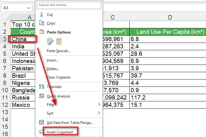
• Etapa 4: Digite seu comentário na caixa de comentário.
• Etapa 5: Clique em qualquer lugar fora da caixa de comentário para finalizar.

O Excel adiciona o comentário à célula selecionada. Se você estiver trabalhando com outras pessoas, elas poderão responder ao comentário e continuar a discussão na mesma conversa.

2. Inserir um Comentário pela Guia Revisão

Você também pode inserir um comentário pela faixa de opções do Excel. Isso é útil quando você já está trabalhando com as ferramentas na guia Revisão.

• Etapa 1: Selecione a célula que deseja comentar.
• Etapa 2: Abra a guia Revisão.
• Etapa 3: Selecione Novo Comentário.

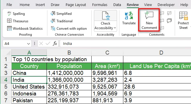
• Etapa 4: Digite os comentários na caixa de comentário.
• Etapa 5: Clique em qualquer lugar fora da caixa de comentário para finalizar.

Essa abordagem proporciona o mesmo resultado básico que usar o menu do botão direito, então você pode usar o fluxo de trabalho que achar mais conveniente.

Dica: Se você também deseja melhorar a aparência geral da sua planilha, pode usar os recursos de formatação integrados do Excel para ajustar rapidamente células, tabelas e outros elementos. Consulte nosso guia sobre Formatação Automática no Excel para mais detalhes.

Como Adicionar Comentários ao Excel com VBA

Os comentários manuais funcionam bem para planilhas pequenas, mas podem se tornar repetitivos quando você precisa adicionar comentários semelhantes a várias células. O VBA permite automatizar esse trabalho diretamente dentro do Excel.

Antes de escrever a macro, você precisa abrir o editor VBA do Excel e criar um módulo. Quando o módulo estiver pronto, você pode colar o código e executá-lo a partir do Excel.

1. Abrir o Editor VBA

• Etapa 1: Abra a pasta de trabalho do Excel que deseja editar.
• Etapa 2: Pressione Alt + F11 para abrir o editor Microsoft Visual Basic for Applications.
• Etapa 3: No editor VBA, selecione Inserir > Módulo.

• Etapa 4: Cole o código VBA no novo módulo.

2. Adicionar um Comentário a uma Célula

Você pode usar VBA para adicionar um comentário a uma célula específica no Excel:

Sub AddComment()

    Range("B4").AddComment "Please review this value."

End Sub

Execute a macro e o Excel adicionará o comentário especificado à célula B4.

3. Adicionar Comentários a Várias Células

Se várias células precisarem de comentários, você pode usar um loop:

Sub AddComments()

    Dim cell As Range

    For Each cell In Range("B4:B8")
        cell.AddComment "Please review this value."
    Next cell

End Sub

Essa abordagem é útil quando o mesmo tipo de comentário precisa ser adicionado em um intervalo.

Observação: O método VBA AddComment está associado ao modelo de comentários mais antigo do Excel. Nas versões atuais do Microsoft 365, o comando mais recente Novo Comentário cria comentários encadeados, enquanto os comentários mais antigos são chamados de anotações.

Como Adicionar Comentários ao Excel com Python

O Python é mais adequado quando a criação de comentários faz parte de um fluxo de trabalho maior de processamento do Excel. Por exemplo, você pode precisar adicionar comentários a arquivos gerados por outro sistema ou processar pastas de trabalho do Excel automaticamente.

Free Spire.XLS para Python fornece APIs para trabalhar com arquivos do Excel sem instalar o Microsoft Excel. Você pode carregar uma pasta de trabalho, acessar uma célula, adicionar um comentário, personalizar sua aparência e salvar o resultado.

1. Instalar o Free Spire.XLS para Python

Instale a biblioteca com o pip:

pip install Spire.Xls.Free

Depois de instalada, você pode usá-la para ler e modificar pastas de trabalho do Excel a partir do Python.

2. Adicionar um Comentário a uma Célula

O exemplo a seguir carrega uma pasta de trabalho existente e adiciona um comentário à célula B4.

from spire.xls import *
from spire.xls.common import *

inputFile = "sample.xlsx"
outputFile = "CommentWithAuthor.xlsx"

# Create a Workbook object
workbook = Workbook()

# Load the Excel workbook
workbook.LoadFromFile(inputFile)

# Get the first worksheet
sheet = workbook.Worksheets[0]

# Get the cell where the comment will be added
cell = sheet.Range["B4"]

# Set the comment author and content
author = "Lucy"
text = "Test comment with author"

# Add a comment to the cell
comment = cell.AddComment()
comment.Text = author + ":\n" + text

# Save the result
workbook.SaveToFile(outputFile, ExcelVersion.Version2013)
workbook.Dispose()

O código primeiro cria um objeto Workbook e carrega o arquivo Excel de origem com LoadFromFile(). Em seguida, obtém a primeira planilha por meio de workbook.Worksheets[0] e usa sheet.Range["B4"] para acessar a célula de destino. Por fim, AddComment() cria um comentário para essa célula, enquanto comment.Text define seu conteúdo antes de a pasta de trabalho modificada ser salva.

3. Personalizar o Comentário

Além de adicionar texto simples na caixa de comentário, você também pode controlar sua aparência. Por exemplo, você pode alterar sua largura e visibilidade e aplicar formatação a parte do texto do comentário.

# Set the comment size and visibility
comment.Width = 200
comment.Visible = True

# Create a font for the author name
font = workbook.CreateFont()
font.FontName = "Segoe Script"
font.KnownColor = ExcelColors.Blue
font.IsBold = True

# Apply the font to the author name
comment.RichText.SetFont(0, len(author), font)

A imagem abaixo mostra o comentário adicionado com este código. Como você pode ver, a caixa de comentário usa uma fonte e uma cor de texto diferentes do formato padrão mostrado na etapa anterior:

Neste pequeno script, Width controla a largura da caixa de comentário, enquanto Visible determina se o comentário é exibido. O objeto RichText permite formatar parte do texto do comentário, como deixar o nome do autor em negrito.

Dica: Depois de saber como adicionar e personalizar comentários com Python, você também pode precisar atualizar ou remover comentários existentes. Consulte nosso guia sobre Editar ou Remover Comentários no Excel para mais detalhes.

Conclusão

Adicionar um comentário no Excel pode ser tão simples quanto selecionar uma célula e escolher Novo Comentário. Se você precisar automatizar tarefas repetitivas de comentários dentro do Excel, o VBA também pode ajudar. Quando você precisa de uma maneira mais eficiente de adicionar comentários de forma programática, o Free Spire.XLS para Python é uma escolha prática. Ele permite adicionar comentários a várias células e personalizar sua aparência com apenas algumas linhas de código. Escolha o método que melhor atende às suas necessidades!

Perguntas Frequentes

Posso Adicionar um Comentário a uma Célula Específica no Excel?

Sim. Selecione a célula, clique com o botão direito nela e escolha Novo Comentário. Você também pode adicionar um comentário pela guia Revisão.

Posso Adicionar Comentários a Várias Células de Uma Só Vez?

Sim. Recomenda-se usar VBA ou Python para automatizar o processo quando várias células precisarem de comentários semelhantes.

Posso Personalizar a Aparência de um Comentário do Excel?

Sim. Com o Free Spire.XLS para Python, você pode ajustar propriedades como a largura e a visibilidade do comentário e aplicar formatação de rich text ao texto do comentário.

Qual É a Diferença Entre um Comentário e uma Anotação no Excel?

No Excel atual, os comentários encadeados são destinados a discussões e respostas, enquanto as anotações são usadas para anotações simples. As anotações eram chamadas de comentários em versões anteriores do Excel.

---

Leia Também:

• Python: Extrair Comentários do Excel
• Como Fazer Tachado no Excel: Métodos para Windows e Mac
• Destacar Duplicatas no Excel: 4 Métodos Fáceis
• Como Excluir Linhas em Branco no Excel: 5 Métodos Fáceis

댓글은 값을 설명하거나, 피드백을 남기거나, 다른 사람과 셀에 대해 논의해야 할 때 유용합니다. Excel에서는 워크시트에서 직접 댓글을 추가하거나, VBA로 프로세스를 자동화하거나, Python을 사용하여 Excel 파일의 댓글을 프로그래밍 방식으로 처리할 수 있습니다. 이 가이드에서는 빠른 수동 방법부터 Free Spire.XLS for Python을 사용한 자동 처리까지, Excel에 댓글을 추가하는 여러 방법을 다룹니다.

• Excel에서 직접 댓글을 추가하는 방법
  • 마우스 오른쪽 버튼 메뉴
  • 검토 탭
• VBA로 Excel에 댓글을 추가하는 방법
• Python으로 Excel에 댓글을 추가하는 방법
• 자주 묻는 질문

Excel에서 직접 댓글을 추가하는 방법

몇 개의 댓글만 추가하면 되는 경우 Excel 자체에서 빠르게 추가할 수 있습니다. 셀의 상황에 맞는 메뉴에서 직접 댓글을 추가하거나 검토 탭을 사용할 수 있습니다. 이러한 방법은 통합 문서를 수동으로 작업하고 많은 셀을 처리할 필요가 없을 때 적합합니다.

1. 마우스 오른쪽 버튼 메뉴에서 댓글 추가

• 1단계: 댓글을 추가할 셀을 선택합니다.
• 2단계: 셀을 마우스 오른쪽 버튼으로 클릭합니다.
• 3단계: 댓글 삽입을 선택합니다.

• 4단계: 댓글 상자에 댓글을 입력합니다.
• 5단계: 완료하려면 댓글 상자 바깥 아무 곳이나 클릭합니다.

Excel은 선택한 셀에 댓글을 추가합니다. 다른 사람과 함께 작업하는 경우, 그들은 댓글에 답장하고 같은 스레드에서 논의를 계속할 수 있습니다.

2. 검토 탭에서 댓글 삽입

Excel 리본에서도 댓글을 삽입할 수 있습니다. 이미 검토 탭의 도구를 사용 중일 때 유용합니다.

• 1단계: 댓글을 달 셀을 선택합니다.
• 2단계: 검토 탭을 엽니다.
• 3단계: 새 댓글을 선택합니다.

• 4단계: 댓글 상자에 댓글을 입력합니다.
• 5단계: 완료하려면 댓글 상자 바깥 아무 곳이나 클릭합니다.

이 방법은 마우스 오른쪽 버튼 메뉴를 사용하는 것과 동일한 기본 결과를 제공하므로, 더 편리하게 느껴지는 워크플로를 사용하면 됩니다.

팁: 워크시트의 전반적인 모양도 개선하고 싶다면 Excel의 기본 제공 서식 기능을 사용하여 셀, 표 및 기타 요소를 빠르게 조정할 수 있습니다. 자세한 내용은 Excel의 자동 서식 가이드를 참조하세요.

VBA로 Excel에 댓글을 추가하는 방법

수동 댓글은 작은 워크시트에서는 잘 작동하지만, 여러 셀에 비슷한 댓글을 추가해야 할 때는 반복적일 수 있습니다. VBA를 사용하면 Excel 내부에서 이 작업을 직접 자동화할 수 있습니다.

매크로를 작성하기 전에 Excel의 VBA 편집기를 열고 모듈을 만들어야 합니다. 모듈이 준비되면 코드를 붙여넣고 Excel에서 실행할 수 있습니다.

1. VBA 편집기 열기

• 1단계: 편집할 Excel 통합 문서를 엽니다.
• 2단계: Alt + F11을 눌러 Microsoft Visual Basic for Applications 편집기를 엽니다.
• 3단계: VBA 편집기에서 삽입 > 모듈을 선택합니다.

• 4단계: 새 모듈에 VBA 코드를 붙여넣습니다.

2. 셀에 댓글 추가

VBA를 사용하여 Excel의 특정 셀에 댓글을 추가할 수 있습니다:

Sub AddComment()

    Range("B4").AddComment "Please review this value."

End Sub

매크로를 실행하면 Excel이 지정된 댓글을 B4 셀에 추가합니다.

3. 여러 셀에 댓글 추가

여러 셀에 댓글이 필요하면 루프를 사용할 수 있습니다:

Sub AddComments()

    Dim cell As Range

    For Each cell In Range("B4:B8")
        cell.AddComment "Please review this value."
    Next cell

End Sub

이 방법은 동일한 유형의 댓글을 범위 전체에 추가해야 할 때 유용합니다.

참고: VBA AddComment 메서드는 Excel의 이전 댓글 모델과 연결되어 있습니다. 현재 Microsoft 365 버전에서는 최신 새 댓글 명령이 스레드된 댓글을 만들며, 이전 댓글은 메모라고 합니다.

Python으로 Excel에 댓글을 추가하는 방법

댓글 생성이 더 큰 Excel 처리 워크플로의 일부인 경우 Python이 더 적합합니다. 예를 들어, 다른 시스템에서 생성된 파일에 댓글을 추가하거나 Excel 통합 문서를 자동으로 처리해야 할 수 있습니다.

Free Spire.XLS for Python은 Microsoft Excel을 설치하지 않고도 Excel 파일로 작업할 수 있는 API를 제공합니다. 통합 문서를 로드하고, 셀에 액세스하고, 댓글을 추가하고, 모양을 사용자 지정하고, 결과를 저장할 수 있습니다.

1. Free Spire.XLS for Python 설치

pip로 라이브러리를 설치합니다:

pip install Spire.Xls.Free

설치가 완료되면 Python에서 Excel 통합 문서를 읽고 수정하는 데 사용할 수 있습니다.

2. 셀에 댓글 추가

다음 예제에서는 기존 통합 문서를 로드하고 B4 셀에 댓글을 추가합니다.

from spire.xls import *
from spire.xls.common import *

inputFile = "sample.xlsx"
outputFile = "CommentWithAuthor.xlsx"

# Create a Workbook object
workbook = Workbook()

# Load the Excel workbook
workbook.LoadFromFile(inputFile)

# Get the first worksheet
sheet = workbook.Worksheets[0]

# Get the cell where the comment will be added
cell = sheet.Range["B4"]

# Set the comment author and content
author = "Lucy"
text = "Test comment with author"

# Add a comment to the cell
comment = cell.AddComment()
comment.Text = author + ":\n" + text

# Save the result
workbook.SaveToFile(outputFile, ExcelVersion.Version2013)
workbook.Dispose()

코드는 먼저 Workbook 개체를 만들고 LoadFromFile()로 원본 Excel 파일을 로드합니다. 그런 다음 workbook.Worksheets[0]을 통해 첫 번째 워크시트를 가져오고 sheet.Range["B4"]를 사용하여 대상 셀에 액세스합니다. 마지막으로 AddComment()가 해당 셀에 대한 댓글을 만들고, comment.Text가 수정된 통합 문서를 저장하기 전에 내용을 설정합니다.

3. 댓글 사용자 지정

댓글 상자에 일반 텍스트를 추가하는 것 외에도 모양을 제어할 수 있습니다. 예를 들어 너비와 표시 여부를 변경하고 댓글 텍스트의 일부에 서식을 적용할 수 있습니다.

# Set the comment size and visibility
comment.Width = 200
comment.Visible = True

# Create a font for the author name
font = workbook.CreateFont()
font.FontName = "Segoe Script"
font.KnownColor = ExcelColors.Blue
font.IsBold = True

# Apply the font to the author name
comment.RichText.SetFont(0, len(author), font)

아래 이미지는 이 코드로 추가된 댓글을 보여 줍니다. 보시다시피 댓글 상자는 이전 단계에 표시된 기본 서식과 다른 글꼴과 텍스트 색을 사용합니다:

이 짧은 스크립트에서 Width는 댓글 상자 너비를 제어하고, Visible은 댓글이 표시되는지 여부를 결정합니다. RichText 개체를 사용하면 작성자 이름을 굵게 표시하는 등 댓글 텍스트의 일부에 서식을 지정할 수 있습니다.

팁: Python으로 댓글을 추가하고 사용자 지정하는 방법을 알게 되면 기존 댓글을 업데이트하거나 제거해야 할 수도 있습니다. 자세한 내용은 Excel에서 댓글 편집 또는 제거 가이드를 참조하세요.

결론

Excel에서 댓글을 추가하는 것은 셀을 선택하고 새 댓글을 선택하는 것만큼 간단할 수 있습니다. Excel 내에서 반복적인 댓글 작업을 자동화해야 한다면 VBA도 도움이 될 수 있습니다. 프로그래밍 방식으로 댓글을 추가하는 더 효율적인 방법이 필요할 때 Free Spire.XLS for Python은 실용적인 선택입니다. 몇 줄의 코드만으로 여러 셀에 댓글을 추가하고 모양을 사용자 지정할 수 있습니다. 필요에 가장 잘 맞는 방법을 선택하세요!

자주 묻는 질문

Excel의 특정 셀에 댓글을 추가할 수 있나요?

예. 셀을 선택하고 마우스 오른쪽 버튼으로 클릭한 다음 새 댓글을 선택합니다. 검토 탭을 통해 댓글을 추가할 수도 있습니다.

여러 셀에 한 번에 댓글을 추가할 수 있나요?

예. 여러 셀에 비슷한 댓글이 필요할 때는 VBA 또는 Python을 사용하여 프로세스를 자동화하는 것이 좋습니다.

Excel 댓글의 모양을 사용자 지정할 수 있나요?

예. Free Spire.XLS for Python을 사용하면 댓글 너비와 표시 여부 같은 속성을 조정하고 댓글 텍스트에 서식 있는 텍스트 서식을 적용할 수 있습니다.

Excel 댓글과 메모의 차이점은 무엇인가요?

현재 Excel에서 스레드된 댓글은 토론과 답장을 위한 것이고, 메모는 간단한 주석에 사용됩니다. 메모는 이전 버전의 Excel에서 댓글이라고 불렸습니다.

---

함께 읽기:

• Python: Excel에서 댓글 추출
• Excel에서 취소선을 적용하는 방법: Windows 및 Mac용 방법
• Excel에서 중복 항목 강조 표시: 4가지 쉬운 방법
• Excel에서 빈 행을 삭제하는 방법: 5가지 쉬운 방법