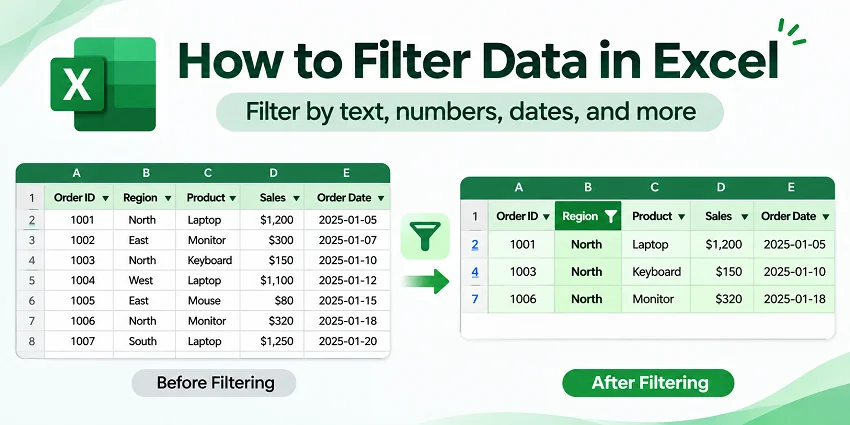
When working with large Excel worksheets, you may need to find specific records without searching through every row. For example, you might want to display orders from a particular region, sales above a certain amount, or transactions within a date range.
Excel lets you filter data based on these conditions without deleting any records. You can also use formulas to extract matching data or Python to automate repetitive filtering tasks.
Quick Answer: How to Filter Data in Excel
To filter data in Excel:
- Select any cell within your dataset.
- Go to Data > Filter to display filter arrows in the column headers.
- Click the arrow in the column you want to filter.
- Select the values you want to display, or choose a condition from Text Filters, Number Filters, or Date Filters.
- Click OK to apply the filter.
Excel displays only the rows that match your criteria. The other rows are hidden, not deleted.
Which Excel Filtering Method Should You Use?
The best approach depends on whether you want to filter the current worksheet, extract matching records, or automate the process.
| Your task | Recommended method | Why use it |
|---|---|---|
| View rows by values, text, numbers, dates, or multiple conditions | AutoFilter | Quick, temporary filtering in the current worksheet |
| Extract matching records into a separate range | FILTER function | Results recalculate when source data changes |
| Apply complex groups of conditions or copy matching records | Advanced Filter | Flexible criteria ranges and a copy-to-location option |
| Apply predefined filters to Excel files automatically | Python | Repeat the same filtering steps without opening Excel |
AutoFilter is also available in Excel for the web, so you can filter worksheets directly in your browser.
Example Excel Dataset
We'll use the following sales data throughout this guide. You can also download the sample Excel workbook to follow along with the examples.
| Order ID | Region | Product | Sales | Order Date |
|---|---|---|---|---|
| 1001 | East | Laptop | 7200 | 2026-01-05 |
| 1002 | West | Monitor | 4300 | 2026-01-11 |
| 1003 | East | Keyboard | 900 | 2026-01-17 |
| 1004 | North | Laptop | 8100 | 2026-02-03 |
| 1005 | South | Monitor | 5200 | 2026-02-10 |
| 1006 | East | Monitor | 6400 | 2026-02-16 |
The data occupies cells A1:E7, including the column headers. The Sales column contains numeric values, and the Order Date column contains actual Excel dates.
You can try each method independently using this workbook.
Method 1: Filter Data Using Excel AutoFilter
Excel's AutoFilter lets you display only the rows that meet your criteria while keeping the remaining data intact. You can filter by specific values, text, numbers, dates, or conditions across multiple columns.
To enable AutoFilter, select any cell within your dataset and go to Data > Filter. Excel adds a filter dropdown to each column header. If your data is already formatted as an Excel Table, these dropdowns are available by default.
Note: Each example below starts with the full dataset unless otherwise stated. Before trying a new example, go to Data > Clear to remove any filters applied previously.
Filter Data by Specific Values
Suppose you want to view only orders from the East region.
- Click the filter arrow in the Region column.
- Uncheck (Select All), then select East.
- Click OK.
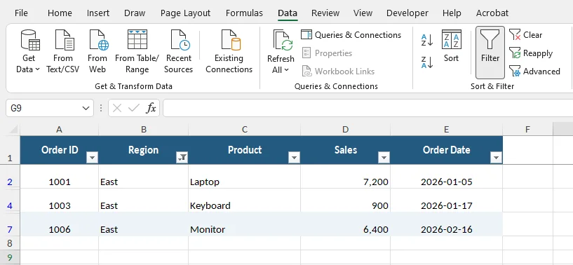
Excel displays only the three matching orders (1001, 1003, and 1006). The other rows are temporarily hidden, but their data remains unchanged.
You can also select multiple values, such as East and West, to display records from either region. For columns with many unique values, use the search box in the filter menu to quickly find specific entries.
Filter Text in Excel
Text Filters help you find records containing specific words or characters. They're useful when filtering product names, customer lists, or other text-based data.
For example, to find products containing "Laptop":
- Click the filter arrow in the Product column.
- Choose Text Filters > Contains.
- In the Custom AutoFilter dialog box, enter
Laptopand click OK.
Excel displays orders 1001 and 1004, both of which have "Laptop" in the Product column.
Other text filter options include Equals, Begins With, Ends With, and Does Not Contain, allowing you to refine your results based on different matching conditions.
Filter Numbers in Excel
Number Filters help you find values above, below, or within a specified range. For example, you can use them to identify orders with sales greater than 5,000.
- Click the filter arrow in the Sales column.
- Choose Number Filters > Greater Than.
- In the Custom AutoFilter dialog box, enter
5000and click OK.
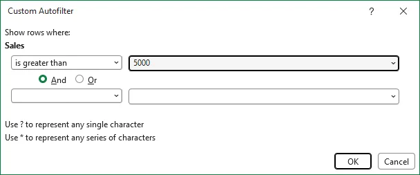
Excel displays four matching orders, with sales amounts of 7,200, 8,100, 5,200, and 6,400.
You can also use Between to include values within a range, Above Average to find values above the column average, or Top 10 to display a selected number of highest or lowest values.
For two custom comparisons in the same column, choose Number Filters > Custom Filter and select And or Or in the dialog box. For example, setting is greater than 5000 And is less than 8000 excludes both boundary values, while Between includes them.
Filter Dates in Excel
Date Filters let you display records from a particular day, month, year, or date range. This is useful when reviewing transaction histories, project schedules, or monthly reports.
For example, to find orders placed during February 2026:
- Click the filter arrow in the Order Date column.
- Choose Date Filters > Between.
- In the Custom AutoFilter dialog box, set the date range from February 1, 2026, to February 28, 2026.
- Click OK.
Excel displays orders 1004, 1005, and 1006.
You can also choose predefined conditions such as Today, This Month, or Last Year, depending on the records you want to review.
Note: Date Filters work when Excel recognizes the values as actual dates. If imported date values are stored as text, Excel may offer Text Filters instead. In that case, convert the text into actual Excel dates before filtering. Simply changing the cells' display format may not convert the underlying text values.
Filter Data by Multiple Criteria
You can apply filters to multiple columns when you need records that satisfy more than one condition.
For example, suppose you want to find orders from the East region with sales greater than 5,000.
- Open the filter menu in the Region column, select only East, and click OK.
- Open the filter menu in the Sales column.
- Choose Number Filters > Greater Than.
- Enter
5000and click OK.
Excel displays two matching orders: 1001 (7,200) and 1006 (6,400).
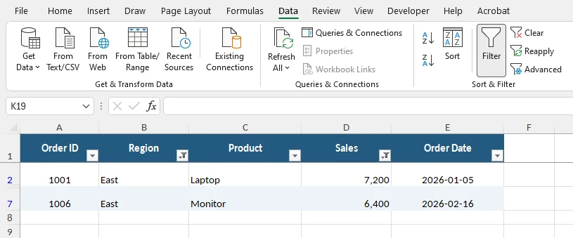
How multiple filter conditions work
When you filter different columns, Excel combines the conditions using AND logic. In this example, each displayed row must satisfy both conditions:
Region = East AND Sales > 5000
Within a single column, selecting multiple values works like an OR condition. For example, selecting East and West displays orders from either region.
If you need OR conditions across different columns, such as finding records where Region is East or Sales exceeds 8,000, the FILTER function or Advanced Filter offers greater flexibility.
After filtering, you can also sort the matching records in Excel by sales amount, date, or other fields to make them easier to review.
Filter by Color or Blank Cells
Excel can also filter data based on cell formatting or missing values.
Filter by color
If you've applied fill or font colors to cells in a column, you can filter that column to display only rows matching a selected color.
- Click the filter arrow in the column containing the formatted cells.
- Select Filter by Color.
- Choose the cell color or font color you want to display.
For example, if you highlight high-priority orders in yellow in the Order ID column, you can filter that column by the yellow fill color.
Filter blank cells
To find records with missing information:
- Click the filter arrow in the relevant column.
- Uncheck (Select All).
- Select (Blanks) and click OK.
Excel displays rows where the selected column contains blank cells.
To try these options with the sample dataset, apply a fill color to a few cells or delete a value from one of the data rows. The (Blanks) option appears only when the selected column contains blank cells.
Filter Data in Excel for the Web
Excel for the web also supports filtering by values, text, numbers, and dates. Open your workbook in the browser, select a cell within your dataset, and go to Data > Filter. You can then use the column filter menus to apply your conditions, much like in desktop Excel.
If you're working on a shared workbook stored in OneDrive or SharePoint, you can use Sheet Views to filter data without affecting how other collaborators see it. Go to View > Sheet View > New and apply your filters. To save the view for later use, select Temporary View from the Sheet View menu, enter a name, and press Enter.
Method 2: Filter Data with the FILTER Function
AutoFilter hides rows that don't match your criteria. If you need to extract matching records into a separate area while keeping the original data visible, the FILTER function is a useful alternative.
The function returns a dynamic array of matching values and recalculates when the referenced data changes. It's available in Excel for Microsoft 365, Excel 2024, Excel 2021, and Excel for the web, but not in Excel 2019 or Excel 2016.
Before trying the examples below, clear any AutoFilter conditions so that all source rows are visible.
Filter Data Based on One Condition
Suppose you want to extract all orders from the East region.
Select an empty cell, such as G2, and enter:
=FILTER(A2:E7,B2:B7="East","No matches")
Press Enter.
Excel returns the three matching records in a separate range, starting at G2.
The formula contains three arguments:
-
A2:E7is the range containing the data to return. -
B2:B7="East"identifies rows where Region equals East. -
"No matches"is the message displayed if no records meet the condition.
The results automatically spill into adjacent cells. You can copy the original column headers to G1:K1 if you want to label the extracted records.
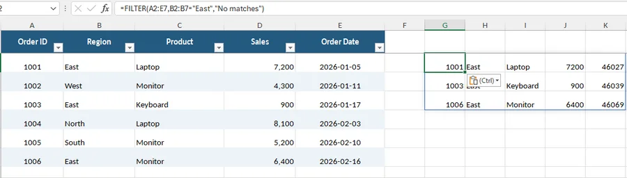
Note: The FILTER function returns values without copying the original cell formatting. If dates in the output appear as serial numbers, select the corresponding output cells and apply a date format using Home > Number Format > Short Date.
Make sure the output area is empty. If existing data blocks the result, Excel may display a #SPILL! error.
Filter Data with Multiple Conditions
The FILTER function can also combine multiple conditions using AND or OR logic.
Example 1: Filter with AND conditions
To extract orders from the East region with sales greater than 5,000, use:
=FILTER(A2:E7,(B2:B7="East")*(D2:D7>5000),"No matches")
The multiplication operator (*) combines the conditions using AND logic. Only orders 1001 and 1006 meet both conditions.
Example 2: Filter with OR conditions
Suppose you want to extract orders where the Region is East or the Sales amount exceeds 8,000.
Use:
=FILTER(A2:E7,(B2:B7="East")+(D2:D7>8000),"No matches")
The addition operator (+) combines the conditions using OR logic. This formula returns orders 1001, 1003, 1004, and 1006 because each record meets at least one condition.
You can also replace a fixed criterion, such as "East", with a cell reference. This lets you change the filtering condition without editing the formula.
Tip: Include new records automatically with an Excel Table
The formulas above use the fixed range A2:E7, so orders added below row 7 won't be included. If your dataset grows regularly, select A1:E7, press Ctrl + T on Windows, confirm that your table has headers, and name it SalesData under Table Design > Table Name.
You can then use structured references:
=FILTER(SalesData,SalesData[Region]="East","No matches")
When you add records to SalesData, its structured references expand automatically, so the FILTER function includes the new matching records. Enter this formula outside the table, and leave enough empty space for its results to spill.
Method 3: Use Advanced Filter for Complex Criteria
Advanced Filter is useful when you need to combine several groups of conditions or copy matching records to another location. Instead of selecting conditions from drop-down menus, you define them in a separate range of worksheet cells.
For example, suppose you want to extract orders that meet either of these requirements:
- Orders from the East region with sales greater than 5,000.
- Orders from the North region with sales greater than 8,000.
The following steps use the desktop version of Excel.
Step 1: Create a Criteria Range
In cells G9:H11, enter the following criteria:
| Region | Sales |
|---|---|
| East | >5000 |
| North | >8000 |
The criteria headers must match the corresponding column headers in your original dataset.
Conditions on the same row use AND logic, while conditions on different rows use OR logic. In this example, Excel will return orders that meet either set of conditions.
Step 2: Apply Advanced Filter
- Select any cell within the original sales dataset.
- Go to Data > Advanced in the Sort & Filter group.
- In the Advanced Filter dialog box, select Copy to another location.
- Enter the following references:
-
List range:
$A$1:$E$7 -
Criteria range:
$G$9:$H$11 -
Copy to:
$J$9
-
List range:
- Click OK.
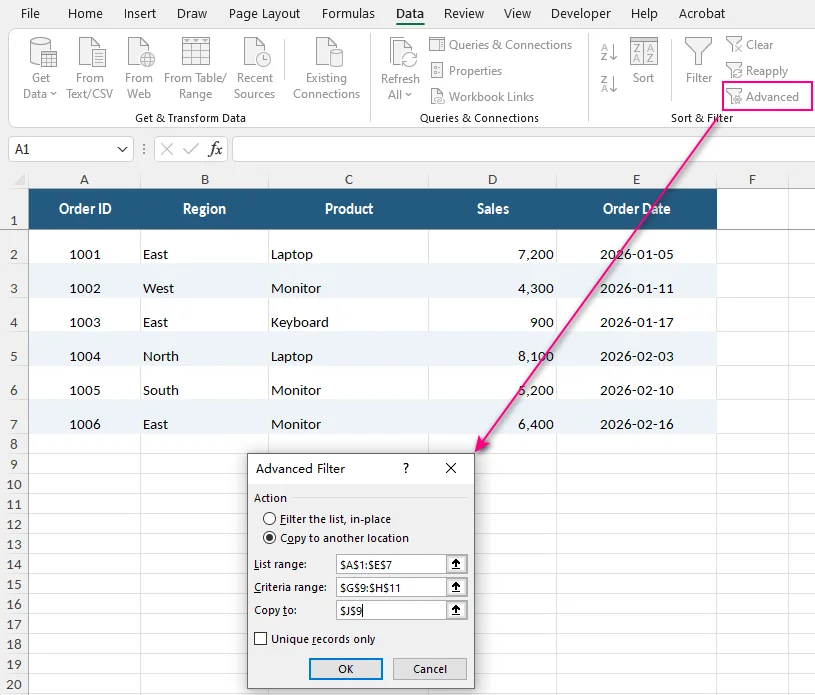
Excel copies orders 1001, 1004, and 1006, along with their column headers, to the destination range starting at J9. The original data remains unchanged.
If you only want to hide rows that don't match, select Filter the list, in-place instead of copying the results.
You can also select Unique records only to exclude duplicate records from the results.
Unlike the FILTER function, Advanced Filter doesn't update the copied results automatically when the source data or criteria change. You need to apply it again to refresh the output.
Method 4: Filter Excel Data Using Python
If you frequently need to apply the same filtering rules to Excel reports, Python can automate the process without requiring you to open and filter each workbook manually.
The following example uses Free Spire.XLS for Python to load an existing workbook, filter the Region column, and save the result without requiring Microsoft Excel.
Step 1: Install the Required Library
Install the free Excel processing library using pip:
pip install Spire.Xls.Free
The free edition supports XLSX files without the worksheet and row limits that apply to the older XLS format.
Step 2: Apply a Filter to an Excel Worksheet
Download sales_data.xlsx and save it in the same folder as your Python script.
The following code loads the workbook, applies an AutoFilter to display only orders from the East region, and saves the filtered result as filtered_sales.xlsx.
from spire.xls import *
from spire.xls.common import *

# Load the Excel workbook
workbook = Workbook()
workbook.LoadFromFile("sales_data.xlsx")

# Access the first worksheet
sheet = workbook.Worksheets[0]

# Set the range to filter
sheet.AutoFilters.Range = sheet.Range["A1:E7"]

# Get the Region filter column (zero-based index 1)
region_filter = sheet.AutoFilters[1]

# Set the filter condition
sheet.AutoFilters.CustomFilter(
    region_filter,
    FilterOperatorType.Equal,
    String("East")
)

# Apply the filter
sheet.AutoFilters.Filter()

# Save the filtered workbook
workbook.SaveToFile("filtered_sales.xlsx", ExcelVersion.Version2016)

# Release resources
workbook.Dispose()
Since Region is the second column, its zero-based filter index is 1. The CustomFilter() method sets the filtering condition, while Filter() applies it.
The same API also supports other filtering scenarios, including date and color filters.
After running the script, open filtered_sales.xlsx to view the results. Only orders 1001, 1003, and 1006 are visible. The other records remain in the workbook and can be displayed again by clearing the filter.
How to Clear or Remove Filters in Excel
To display all records again, go to Data > Clear. This removes the active filter conditions while keeping the filter buttons available.
You can also clear an individual column's filter by opening its filter menu and choosing Clear Filter From "Column Name". To turn off AutoFilter for a standard data range, select a cell within the range and click Data > Filter.
If you need to remove filters from multiple worksheets or automate the process, Excel also supports other ways to clear or remove filters.
Troubleshooting Common Excel Filter Problems
1. Why Is Excel Not Filtering All Rows?
Possible cause: Blank rows or columns may cause Excel to detect only part of your dataset.
How to fix: Select the entire data range, including the column headers, before enabling filtering. Alternatively, convert the range into an Excel Table using Ctrl + T on Windows.
If you've added new records, make sure they're included in the filter range. If existing values have changed but the filtered results haven't updated, go to Data > Reapply to refresh them.
2. Why Are Number or Date Filters Missing in Excel?
Possible cause: Some values may be stored as text rather than actual numbers or dates.
For example, if the Sales column contains a mixture of numbers and text-formatted numbers, Excel may display Text Filters instead of Number Filters.
How to fix: Check the underlying cell values and convert incorrectly stored numbers or dates to their appropriate data types.
Simply changing the cells' number format doesn't always convert text into actual numbers or dates.
3. Why Does the FILTER Function Return a #SPILL! Error?
Possible cause: The formula's output range contains existing data or merged cells, preventing the result from expanding.
How to fix: Move the formula to an empty area, clear any cells blocking its output, or unmerge cells where necessary.
Also, enter dynamic array formulas outside Excel Tables, since spilled array results cannot expand within table cells.
4. Why Are Some Rows Still Hidden After Clearing Filters?
Possible cause: The rows may have been hidden manually rather than through a filter.
How to fix: Select the surrounding row headers, right-click, and choose Unhide.
Clearing filter conditions restores rows hidden by filtering, but it doesn't automatically unhide manually hidden rows.
Conclusion
Excel offers several ways to filter data depending on your needs. AutoFilter is ideal for everyday filtering, while the FILTER function creates dynamic results that update when the source data changes. Advanced Filter handles more complex criteria, and Python helps automate repetitive filtering tasks across Excel reports.
For reliable results, keep your data organized, use consistent data types, and make sure your filter ranges include all relevant records.