Create Excel Scatter Chart in C#

Charts are used to display series of numeric data in a graphical format to make it easier to understand large quantities of data and the relationship between different series of data. This article talks about how to create scatter chart via Spire.XLS.

To create a Scatter Chart, execute the following steps.

Step 1: Create a new Excel document and get the first sheet.

Workbook workbook = new Workbook();
workbook.CreateEmptySheets(1);
Worksheet sheet = workbook.Worksheets[0];

Step 2: Rename the first sheet and set the grid lines invisible.

sheet.Name = "Scatter Chart";
sheet.GridLinesVisible = false;

Step 3: Create a scatter chart and set data region for it.

Chart chart = sheet.Charts.Add(ExcelChartType.ScatterMarkers);
chart.DataRange = sheet.Range["B2:B10"];
chart.SeriesDataFromRange = false;

Step 4: Set position and title for the chart.

chart.LeftColumn = 1;
chart.TopRow = 6;
chart.RightColumn = 9;
chart.BottomRow = 25;

chart.ChartTitle = "Scatter Chart";
chart.ChartTitleArea.IsBold = true;
chart.ChartTitleArea.Size = 12;

Step 5: Add data to the excel range.

sheet.Range["A1"].Value = "Y(Salary)";
sheet.Range["A2"].Value = "42763";
sheet.Range["A3"].Value = "195387";
sheet.Range["A4"].Value = "35672";
sheet.Range["A5"].Value = "217637";
sheet.Range["A6"].Value = "74734";
sheet.Range["A7"].Value = "130550";
sheet.Range["A8"].Value = "42976";
sheet.Range["A9"].Value = "15132";
sheet.Range["A10"].Value = "54936";

sheet.Range["B1"].Value = "X(Car Price)";
sheet.Range["B2"].Value = "19455";
sheet.Range["B3"].Value = "93965";
sheet.Range["B4"].Value = "20858";
sheet.Range["B5"].Value = "107164";
sheet.Range["B6"].Value = "34036";
sheet.Range["B7"].Value = "87806";
sheet.Range["B8"].Value = "17927";
sheet.Range["B9"].Value = "61518";
sheet.Range["B10"].Value = "29479";

Step 6: Set style color for the range.

sheet.Range["A2:B2"].Style.KnownColor = ExcelColors.LightOrange;
sheet.Range["A3:B3"].Style.KnownColor = ExcelColors.LightYellow;
sheet.Range["A4:B4"].Style.KnownColor = ExcelColors.LightOrange;
sheet.Range["A5:B5"].Style.KnownColor = ExcelColors.LightYellow;
sheet.Range["A6:B6"].Style.KnownColor = ExcelColors.LightOrange;
sheet.Range["A7:B7"].Style.KnownColor = ExcelColors.LightYellow;
sheet.Range["A8:B8"].Style.KnownColor = ExcelColors.LightOrange;
sheet.Range["A9:B9"].Style.KnownColor = ExcelColors.LightYellow;
sheet.Range["A10:B10"].Style.KnownColor = ExcelColors.LightOrange;

Step 7: Set number format for cell ranges.

sheet.Range["A2:B10"].Style.NumberFormat = "\"$\"#,##0";

Step 8: Set data for axis x y.

chart.Series[0].CategoryLabels = sheet.Range["A2:A10"];
chart.Series[0].Values = sheet.Range["B2:B10"];

Step 9: Add a trend line.

chart.Series[0].TrendLines.Add(TrendLineType.Exponential);

Step 10: Add axis title.

chart.PrimaryValueAxis.Title = "Salary";
chart.PrimaryCategoryAxis.Title = "Car Price";

Step 11: Save and review.

workbook.SaveToFile("XYChart.xlsx", FileFormat.Version2013);
System.Diagnostics.Process.Start("XYChart.xlsx");

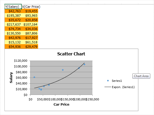
Screenshot:

Create Excel Scatter Chart in C#

Full code:

using Spire.Xls;
namespace CreateExcelScatterChart
{
    class Program
    {

        static void Main(string[] args)
        {
            Workbook workbook = new Workbook();
            workbook.CreateEmptySheets(1);
            Worksheet sheet = workbook.Worksheets[0];

            sheet.Name = "Scatter Chart";
            sheet.GridLinesVisible = false;

            Chart chart = sheet.Charts.Add(ExcelChartType.ScatterMarkers);
            chart.DataRange = sheet.Range["B2:B10"];
            chart.SeriesDataFromRange = false;

            chart.LeftColumn = 1;
            chart.TopRow = 6;
            chart.RightColumn = 9;
            chart.BottomRow = 25;

            chart.ChartTitle = "Scatter Chart";
            chart.ChartTitleArea.IsBold = true;
            chart.ChartTitleArea.Size = 12;

            sheet.Range["A1"].Value = "Y(Salary)";
            sheet.Range["A2"].Value = "42763";
            sheet.Range["A3"].Value = "195387";
            sheet.Range["A4"].Value = "35672";
            sheet.Range["A5"].Value = "217637";
            sheet.Range["A6"].Value = "74734";
            sheet.Range["A7"].Value = "130550";
            sheet.Range["A8"].Value = "42976";
            sheet.Range["A9"].Value = "15132";
            sheet.Range["A10"].Value = "54936";

            sheet.Range["B1"].Value = "X(Car Price)";
            sheet.Range["B2"].Value = "19455";
            sheet.Range["B3"].Value = "93965";
            sheet.Range["B4"].Value = "20858";
            sheet.Range["B5"].Value = "107164";
            sheet.Range["B6"].Value = "34036";
            sheet.Range["B7"].Value = "87806";
            sheet.Range["B8"].Value = "17927";
            sheet.Range["B9"].Value = "61518";
            sheet.Range["B10"].Value = "29479";

            sheet.Range["A2:B2"].Style.KnownColor = ExcelColors.LightOrange;
            sheet.Range["A3:B3"].Style.KnownColor = ExcelColors.LightYellow;
            sheet.Range["A4:B4"].Style.KnownColor = ExcelColors.LightOrange;
            sheet.Range["A5:B5"].Style.KnownColor = ExcelColors.LightYellow;
            sheet.Range["A6:B6"].Style.KnownColor = ExcelColors.LightOrange;
            sheet.Range["A7:B7"].Style.KnownColor = ExcelColors.LightYellow;
            sheet.Range["A8:B8"].Style.KnownColor = ExcelColors.LightOrange;
            sheet.Range["A9:B9"].Style.KnownColor = ExcelColors.LightYellow;
            sheet.Range["A10:B10"].Style.KnownColor = ExcelColors.LightOrange;

            sheet.Range["A2:B10"].Style.NumberFormat = "\"$\"#,##0";

            chart.Series[0].CategoryLabels = sheet.Range["A2:A10"];
            chart.Series[0].Values = sheet.Range["B2:B10"];

            chart.Series[0].TrendLines.Add(TrendLineType.Exponential);

            chart.PrimaryValueAxis.Title = "Salary";
            chart.PrimaryCategoryAxis.Title = "Car Price";

            workbook.SaveToFile("XYChart.xlsx", FileFormat.Version2013);
            System.Diagnostics.Process.Start("XYChart.xlsx");
        }
    }
}

Create Excel Scatter Chart in C#

See Also